
Estimate of marginal ("main") effects instead of ANOVA for factorial experiments
keywords: estimation, ANOVA, factorial, model simplification, conditional effects, marginal effects
Background
I recently read a paper from a very good ecology journal that communicated the results of an ANOVA like that below (Table 1) using a statement similar to “The removal of crabs strongly decreased algae cover (\(F_{1,36} = 17.4\), \(p < 0.001\))” (I’ve made the data for this table up. The actual experiment had nothing to do with crabs or algae).
| Df | F value | Pr(>F) | |
|---|---|---|---|
| snail | 36 | 26.7 | 0.000009 |
| crab | 36 | 17.4 | 0.000182 |
| snail:crab | 36 | 16.1 | 0.000290 |
This is a Type III ANOVA table, so the “crab” term in the ANOVA table is a “main” effect, which can be thought of as the average of the effects of crab removal at low snail density and at high snail density1. It’s not wrong to say “crab removal reduced algae cover” but it is misleading if not meaningless. Because it’s an average, a main effect is hard to interpret without looking at the values going into that average, which can be inspected with a plot.
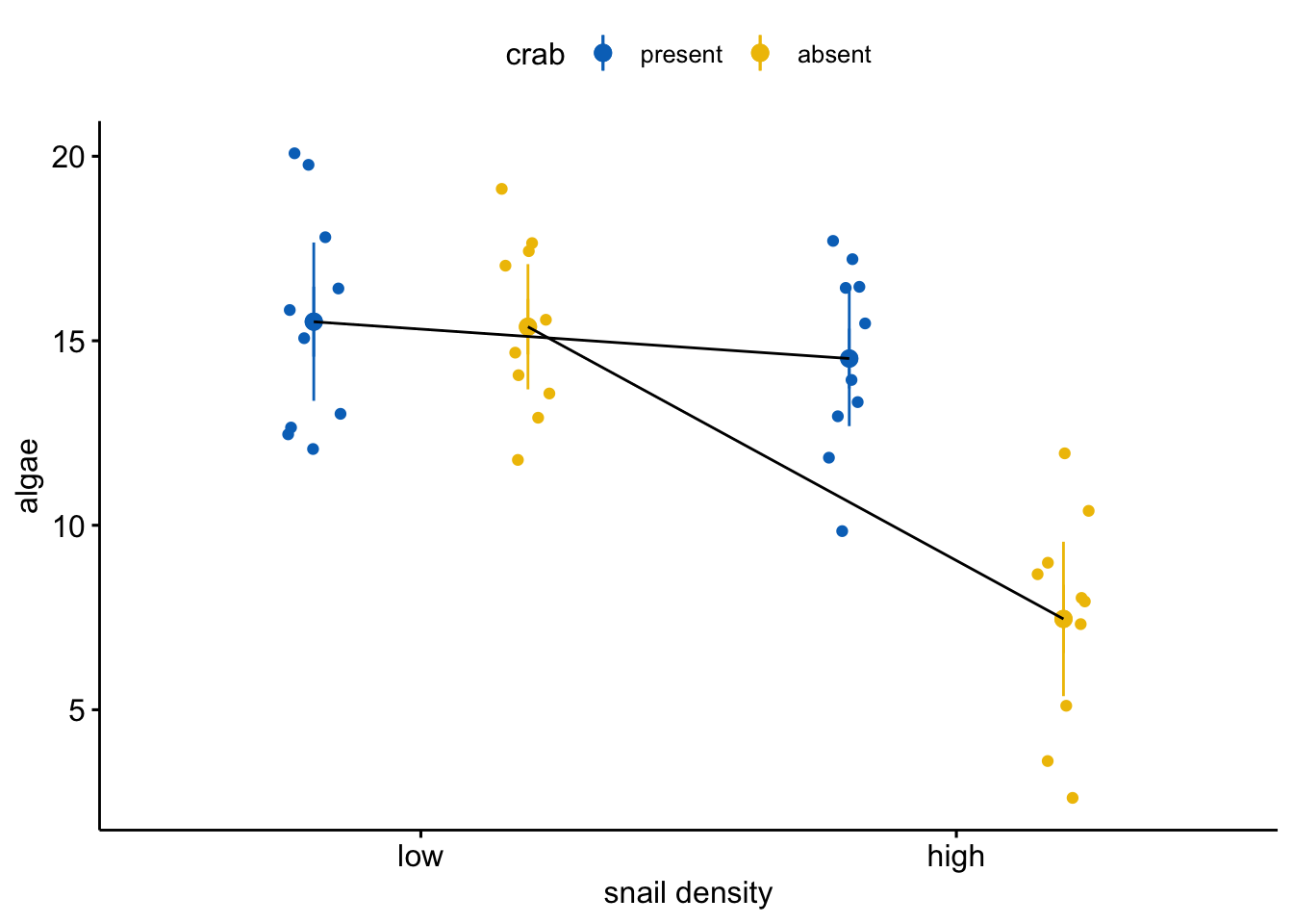
The plot shows a large interaction – the observed effect of crab removal is large when snail density is high but small when snail density is low 2. It is very misleading to conclude that crab removal decreases algae cover when the data support this conclusion only when snail density is high. It’s not wrong – the average effect is decreased algae – but I don’t think the average effect has much meaning here.
I’ve heard two general rules of thumb for interpreting main effects of an ANOVA table: 1) if there is a significant interaction, do not interpret the main effects, and 2) only interpret the main effects after looking at the plot. I explore these below in “When to estimate marginal effects”. A more important question that this example raises is, Do ANOVA tables encourage this kind of misleading interpretation and communication? On most days, I woud say “yes.” And this raises a second question: Would we have similar misleading interpretations if researchers used an estimation approach to analysis instead of ANOVA/testing approach?
Motivated by these questions, this doodle has two parts. In part one, I compare the mapping of the estimation of marginal effects of a factorial design to inference from the “main” effects of an ANOVA table. The second part probes the questions, why/when would we even want to estimate marginal effects?
The motivation is, more generally, the great majority of papers that I read in experimental ecology/evolution while looking for motivating examples and data to teach.
- In many of these articles, the researchers interpret the main effects terms of a full-factorial ANOVA table computed from Type III sums of squares (a practice that is highly controversial among statisticians). These may be followed up with estimates of conditional effects but this is much less common that I would expect (and wish)
- Much less commonly, researchers interpret the main effects term of the ANOVA table refit with only additive terms (or Type II sums of squares).
But why ANOVA (other than it was easy to compute 60 years ago without a computer). Why not simply estimate relevant contrasts? If the design is factorial, the relevant contrasts are generally the conditional effects (or “simple” effects) but could be the marginal effects computed from the additive model (marginal effects are computed as contrasts of marginal means). The advantage of estimation over ANOVA is that estimates and uncertainty matter (how can we predict the consequences of CO2 and warming with F statistics and p-values)
Comparing marginal effects to main effect terms in an ANOVA table
First, some fake data
set.seed(1)
n <- 10

# get random error
sigma <- 2.5

snail_levels <- c("low","high")
crab_levels <- c("present", "absent")
fake_data <- data.table(
  snail = factor(rep(snail_levels, each=n*2),
                snail_levels),
  crab = factor(rep(rep(crab_levels, each=n), 2), crab_levels)
)
X <- model.matrix(~snail*crab, data=fake_data)
beta <- c(15, -3.5, 1.5, -3)

# find a pretty good match of parameters
done <- FALSE
seed_i <- 0
tol <- 0.1
while(done==FALSE){
  seed_i <- seed_i + 1
  set.seed(seed_i)
  epsilon <- rnorm(n*2*2, sd=sigma)
  fake_data[, algae := (X%*%beta)[,1] + epsilon]
  fit <- lm(algae ~ snail*crab, data=fake_data)
  coef_i <- coef(fit)
  if(abs(coef_i[2] - beta[2]) < tol &
     abs(coef_i[3] - beta[3]) < tol &
     abs(coef_i[4] - beta[4]) < tol){done <- TRUE}
}

# the fake data
set.seed(seed_i)
epsilon <- rnorm(n*2*2, sd=sigma)
fake_data[, algae := (X%*%beta)[,1] + epsilon]
Coefficients of the model
fit <- lm(algae ~ snail*crab, data=fake_data)
coef(summary(fit))
## Estimate Std. Error t value Pr(>|t|)
## (Intercept) 15.517280 0.8621397 17.998568 1.391597e-19
## snailhigh -3.498986 1.2192496 -2.869786 6.834572e-03
## crababsent 1.562369 1.2192496 1.281418 2.082394e-01
## snailhigh:crababsent -2.919097 1.7242794 -1.692937 9.910554e-02Conditional (simple) effects
fit.emm <- emmeans(fit, specs=c("snail", "crab"))
fit.pairs <- contrast(fit.emm,
                      method="revpairwise",
                      simple="each",
                      combine=TRUE,
                      adjust="none")
knitr::kable(summary(fit.pairs), digits=c(0,0,0,2, 2, 0, 2, 3))| crab | snail | contrast | estimate | SE | df | t.ratio | p.value |
|---|---|---|---|---|---|---|---|
| present | . | high - low | -3.50 | 1.22 | 36 | -2.87 | 0.007 |
| absent | . | high - low | -6.42 | 1.22 | 36 | -5.26 | 0.000 |
| . | low | absent - present | 1.56 | 1.22 | 36 | 1.28 | 0.208 |
| . | high | absent - present | -1.36 | 1.22 | 36 | -1.11 | 0.273 |
What the data look like
set.seed(1)
pd <- position_dodge(0.8)
gg_response <- ggerrorplot(
  x = "snail",
  y = "algae",
  color = "crab",
  add = c("mean_ci", "jitter"),
  alpha=0.5,
  position = pd,
  palette = "jco",
  data = fake_data
) +
  #geom_point(data=fit.emm, aes(x=snail, y=emmean, fill=crab),
  #          position=pd, size=3) +
  geom_line(data=summary(fit.emm), aes(x=snail, y=emmean, group=crab),
            position=pd) +
  NULL

gg_response
Comparison of marginal effects vs. “main” effects term of ANOVA table when data are balanced
m1 <- lm(algae ~ snail*crab, data=fake_data)
m2 <- lm(algae ~ snail + crab, data=fake_data)
m1_emm <- emmeans(m1, specs="snail")
m2_emm <- emmeans(m2, specs="snail")
m1_marginal <- contrast(m1_emm, method="revpairwise", adjust="none")
m2_marginal <- contrast(m2_emm, method="revpairwise", adjust="none")

con3 <- list(snail=contr.sum, crab=contr.sum)
m3 <- lm(algae ~ snail*crab, data=fake_data, contrasts=con3)
m4 <- lm(algae ~ snail + crab, data=fake_data, contrasts=con3)
m3_coef <- coef(summary(m3))
m4_coef <- coef(summary(m4))
m3_anova <- Anova(m3, type="3")
m4_anova <- Anova(m4, type="3")

# res_table <- data.table(" "=c("Estimate", "SE", "df", "statistic", "p-value"),
#   "marginal (full)"=unlist(summary(m1_marginal)[1, c(2:6)]),
#   "ANOVA (full)"=c(NA, NA, round(m3_anova["Residuals", "Df"],0), unlist(m3_anova[2, 3:4])),
#   "marginal (add)"=unlist(summary(m2_marginal)[1, c(2:6)]),
#   "ANOVA (add)"=c(NA, NA, round(m4_anova["Residuals", "Df"],0), unlist(m4_anova[2, 3:4]))
# )

col_names <- c("Estimate", "SE", "df", "statistic", "p-value")
row_names <- c("marginal (full)", "marginal (add)", "ANOVA (full)", "ANOVA (add)")
res_table <- data.table(t(matrix(c(
  unlist(summary(m1_marginal)[1, c(2:6)]),
  unlist(summary(m2_marginal)[1, c(2:6)]),
  c(NA, NA, round(m3_anova["Residuals", "Df"],0), unlist(m3_anova[2, 3:4])),
  c(NA, NA, round(m4_anova["Residuals", "Df"],0), unlist(m4_anova[2, 3:4]))),
  nrow=5, ncol=4
)))
setnames(res_table, old=colnames(res_table), new=col_names)
res_table <- cbind(method=row_names, res_table)

knitr::kable(res_table, digits=5, caption="Marginal effects of Snail (pooled across levels of crab) computed from the full-factorial and additive models. ANOVA columns are from the Snail term of the ANOVA table from the full-factorial and additive models")| method | Estimate | SE | df | statistic | p-value |
|---|---|---|---|---|---|
| marginal (full) | -4.95853 | 0.86214 | 36 | -5.75143 | 0 |
| marginal (add) | -4.95853 | 0.88361 | 37 | -5.61166 | 0 |
| ANOVA (full) | NA | NA | 36 | 33.07892 | 0 |
| ANOVA (add) | NA | NA | 37 | 31.49073 | 0 |
Comparison of marginal effects vs. “main” effects term of ANOVA table when data are unbalanced
Delete some data
set.seed(1)
inc <- c(1:10,
         sample(11:20, 6),
         sample(21:30, 8),
         sample(31:40, 5))
fake_data_missing <- fake_data[inc,]
knitr::kable(fake_data_missing[, .(N=.N), by=c("snail", "crab")])| snail | crab | N |
|---|---|---|
| low | present | 10 |
| low | absent | 6 |
| high | present | 8 |
| high | absent | 5 |
Marginal effects v ANOVA table main effects
m0 <- lm(algae ~ snail, data=fake_data_missing)
m1 <- lm(algae ~ snail*crab, data=fake_data_missing)
m2 <- lm(algae ~ snail + crab, data=fake_data_missing)
m1_emm <- emmeans(m1, specs="snail")
m2_emm <- emmeans(m2, specs="snail")
m1_marginal <- contrast(m1_emm, method="revpairwise", adjust="none")
m2_marginal <- contrast(m2_emm, method="revpairwise", adjust="none")

con3 <- list(snail=contr.sum, crab=contr.sum)
m3 <- lm(algae ~ snail*crab, data=fake_data_missing, contrasts=con3)
m4 <- lm(algae ~ snail + crab, data=fake_data_missing, contrasts=con3)
m3_coef <- coef(summary(m3))
m4_coef <- coef(summary(m4))
m3_anova <- Anova(m3, type="3")
m4_anova <- Anova(m4, type="3")
m4_anova_2 <- Anova(m4, type="2")
m2_anova_2 <- Anova(m2, type="2")
m3_anova_2 <- Anova(m3, type="2")

# res_table <- data.table(" "=c("Estimate", "SE", "df", "statistic", "p-value"),
#   "marginal (full)"=unlist(summary(m1_marginal)[1, c(2:6)]),
#   "ANOVA (full)"=c(NA, NA, round(m3_anova["Residuals", "Df"],0), unlist(m3_anova[2, 3:4])),
#   "marginal (add)"=unlist(summary(m2_marginal)[1, c(2:6)]),
#   "ANOVA (add)"=c(NA, NA, round(m4_anova["Residuals", "Df"],0), unlist(m4_anova[2, 3:4]))
# )

col_names <- c("Estimate", "SE", "df", "statistic", "p-value")
row_names <- c("marginal (full)", "marginal (add)", "ANOVA (full)", "ANOVA (add)")
res_table <- data.table(t(matrix(c(
  unlist(summary(m1_marginal)[1, c(2:6)]),
  unlist(summary(m2_marginal)[1, c(2:6)]),
  c(NA, NA, round(m3_anova["Residuals", "Df"],0), unlist(m3_anova[2, 3:4])),
  c(NA, NA, round(m4_anova["Residuals", "Df"],0), unlist(m4_anova[2, 3:4]))),
  nrow=5, ncol=4
)))
setnames(res_table, old=colnames(res_table), new=col_names)
res_table <- cbind(method=row_names, res_table)

knitr::kable(res_table, digits=5, caption="Marginal effects of Snail (pooled across levels of crab) computed from the full-factorial and additive models. ANOVA columns are from the Snail \"main effect\" term of the ANOVA table from the full-factorial and additive models")| method | Estimate | SE | df | statistic | p-value |
|---|---|---|---|---|---|
| marginal (full) | -5.71571 | 1.01894 | 25 | -5.60946 | 1e-05 |
| marginal (add) | -5.32370 | 1.01895 | 26 | -5.22469 | 2e-05 |
| ANOVA (full) | NA | NA | 25 | 31.46601 | 1e-05 |
| ANOVA (add) | NA | NA | 26 | 27.29736 | 2e-05 |
Different ways of computing marginal effects in R
- Marginal effects of additive model from emmeans (dummy coding)
- Type II ANOVA of additive model from car (dummy coding)
- Type II ANOVA of additive model from car (effects coding)
- Type III ANOVA of additive model from car (effects coding)
- Type II ANOVA of factorial model from car (effects coding)
col_names <- c("Estimate", "SE", "df", "statistic", "p-value")
row_names <- c("1. marginal effects (additive, dummy coding)",
               "2. Type 2 ANOVA (additive, dummy coding)",
               "3. Type 2 ANOVA  (additive, effects coding)",
               "4. Type 3 ANOVA  (additive, effects coding)",
               "5. Type 2 ANOVA  (full, effects coding)")
type_2_table <- data.table(t(matrix(c(
  unlist(summary(m2_marginal)[1, c(2:6)]),
  c(NA, NA, round(m2_anova_2["Residuals", "Df"],0), unlist(m2_anova_2[1, 3:4])),
  c(NA, NA, round(m4_anova_2["Residuals", "Df"],0), unlist(m4_anova_2[1, 3:4])),
  c(NA, NA, round(m4_anova["Residuals", "Df"],0), unlist(m4_anova[2, 3:4])),
  c(NA, NA, round(m3_anova_2["Residuals", "Df"],0), unlist(m3_anova_2[1, 3:4]))),
  nrow=5, ncol=5
)))
setnames(type_2_table, old=colnames(type_2_table), new=col_names)
type_2_table <- cbind(method=row_names, type_2_table)

knitr::kable(type_2_table)| method | Estimate | SE | df | statistic | p-value |
|---|---|---|---|---|---|
| 1. marginal effects (additive, dummy coding) | -5.323701 | 1.018951 | 26 | -5.224687 | 1.86e-05 |
| 2. Type 2 ANOVA (additive, dummy coding) | NA | NA | 26 | 27.297359 | 1.86e-05 |
| 3. Type 2 ANOVA (additive, effects coding) | NA | NA | 26 | 27.297359 | 1.86e-05 |
| 4. Type 3 ANOVA (additive, effects coding) | NA | NA | 26 | 27.297359 | 1.86e-05 |
| 5. Type 2 ANOVA (full, effects coding) | NA | NA | 25 | 28.958022 | 1.39e-05 |
When to estimate marginal effects
Interactions effects are ubiquitous if not universal. Consequently, the decision to estimate and present marginal effects, as opposed to conditional effects, should not be in the service of a futile effort to learn the “true” model but should depend only on how much one wants to simplify a working model of a system.
I would tend to not estimate marginal effects given the data analyzed above. The data are noisy but are compatible with an interesting interaction and, consequently, an interesting pattern of conditional effects. Namely, the effect of crab removal decreases algae cover when snail density is high but increases algae cover when snail density is low. Again, the data are too noisy to estimate the effects with much certainty, and good practice would be a set of replication experiments to estimate these effects with more precision. If the model were reduced and only the marginal effects were estimated, the possibility of this more complex model of how the system functions would be masked.
The data in the right side of the figure below are precisely those in the analysis above (and reproduced in the left figure below) except the effect of crab removal (at the reference level of snail) is changed from +1.5 to -5. The effect of increasing snail density is the same. The interaction is the same. The residuals are the same.
Even though the interaction effect is the same as that above, relative to the treatment effects of both snail density and crab removal, it is relatively small. Consequently at both levels of snail density, crab removal results in large decrease in algae cover. As long as we don’t have any theory that is quantitative enough to predict this pattern, there is not much loss of understanding if we simply reduce this to the additive model. We don’t claim in the paper that “there is no interaction” or that the effects of crab removal are the same at both levels of snail density, but only that the reduced model and the computation of the marginal effects is a good “working model” of what is going on.
#beta <- c(15, -3.5, 1.5, -3)
beta2 <- c(15, -3.5, -5, -3)
fake_data[, algae2 := (X%*%beta2)[,1] + epsilon]

fit <- lm(algae2 ~ snail*crab, data=fake_data)
coef(summary(fit))
## Estimate Std. Error t value Pr(>|t|)
## (Intercept) 15.517280 0.8621397 17.998568 1.391597e-19
## snailhigh -3.498986 1.2192496 -2.869786 6.834572e-03
## crababsent -4.937631 1.2192496 -4.049730 2.606853e-04
## snailhigh:crababsent -2.919097 1.7242794 -1.692937 9.910554e-02fit.emm <- emmeans(fit, specs=c("snail", "crab"))
fit.pairs <- contrast(fit.emm,
method="revpairwise",
simple="each",
combine=TRUE,
adjust="none")
knitr::kable(summary(fit.pairs), digits=c(0,0,0,2, 2, 0, 2, 3))| crab | snail | contrast | estimate | SE | df | t.ratio | p.value |
|---|---|---|---|---|---|---|---|
| present | . | high - low | -3.50 | 1.22 | 36 | -2.87 | 0.007 |
| absent | . | high - low | -6.42 | 1.22 | 36 | -5.26 | 0.000 |
| . | low | absent - present | -4.94 | 1.22 | 36 | -4.05 | 0.000 |
| . | high | absent - present | -7.86 | 1.22 | 36 | -6.44 | 0.000 |
set.seed(1)
pd <- position_dodge(0.8)
gg_response_2 <- ggerrorplot(
  x = "snail",
  y = "algae2",
  color = "crab",
  add = c("mean_ci", "jitter"),
  alpha=0.5,
  position = pd,
  palette = "jco",
  data = fake_data
) +
  #geom_point(data=fit.emm, aes(x=snail, y=emmean, fill=crab),
  #          position=pd, size=3) +
  geom_line(data=summary(fit.emm), aes(x=snail, y=emmean, group=crab),
            position=pd) +
  NULL


plot_grid(gg_response, gg_response_2)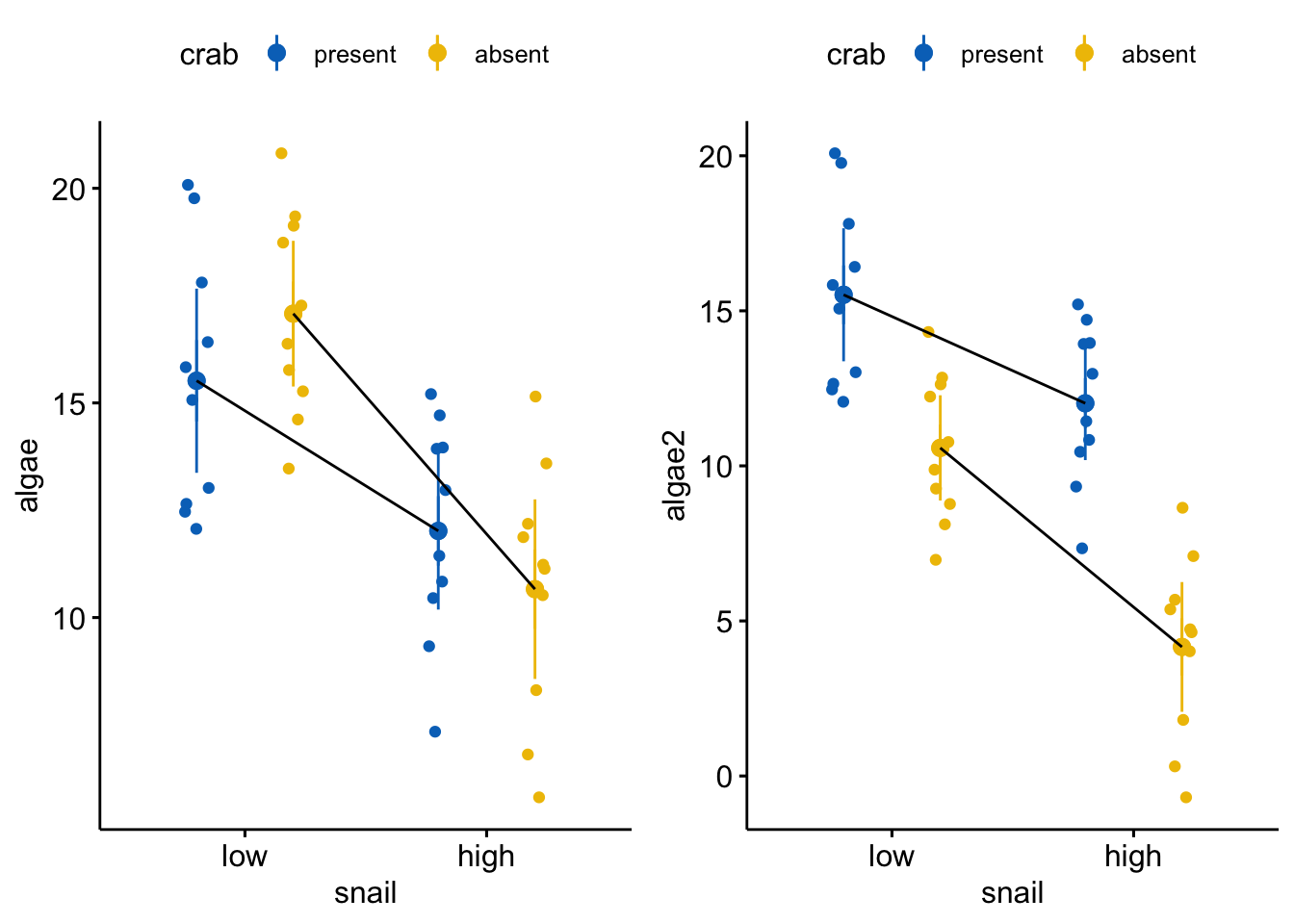
the sum of squares is based on marginal means, so the effect is really a difference in marginal means↩
This interaction shows up in the ANOVA table but its magnitude is impossible to reconstruct from an F-ratio or p-value. Regardless, the average is intermediate, but big enough to result in a very small p-value in the ANOVA table.↩
