
Bootstrap confidence intervals when sample size is really small
TL;DR
A sample table from the full results for data that look like this
| parameter | n=5 | n=10 | n=20 | n=40 | n=80 |
|---|---|---|---|---|---|
| means | |||||
| Control | 81.4 | 87.6 | 92.2 | 93.0 | 93.6 |
| b4GalT1-/- | 81.3 | 90.2 | 90.8 | 93.0 | 93.8 |
| difference in means | |||||
| diff | 83.3 | 87.9 | 91.8 | 92.9 | 93.8 |
Bootstrap CIs are extremely optimistic (too narrow) with data that look like the modeled data when n is 5 (coverage of a 95% interval is 81-83%) and remain optimistic even at n=20, which is a uncommonly large sample size in many bench biology experiments. This result convinces me that the bootstrap should not be generally recommended.
Background
This is part II of how to represent uncertainty in the mean response of each treatment level. A 1 SE bar, where the SE is computed for each group independently, is nearly universal in much of biology. Part I explains why I prefer confidence intervals to SE bars and explores several alternative methods for computing a CI. One alternative is a non-parametric bootstrap. I like the bootstrap – it is extremely useful for learning and teaching what “frequentist” means. It is not dependent on any distribution. It can be used to compute CIs for statistics where no parametric CI exists. And its (fairly) easy to implement!
I am embarrassed to admit that I don’t know how well bootstrap CIs perform with really small sample sizes, say 5 or 10, which are common in experimental (and especially wet-bench) biology. By “perform”, I mean coverage – the actual number of intervals that contain the parameter (true value). If the nominal value is 95% and the coverage is 80%, our results aren’t what we think they are. Part of my ignorance is because the focus on on errors related to the presence of an effect (Type I, Power, FDR) and not on errors related to the magnitude of an effect (Type “S”, Type “M”, coverage of CIs). But part of my ignorance is also because I just don’t recall any source making a big deal about any issues with bootstrap CIs for small samples, at least in the “how-to” literature and not technical literature (like books explicitly on the bootstrap)
The question pursued here is, what is the coverage (the actual frequency of intervals that include the statistic) of a bootstrap interval for really small samples sizes…on the order of n = 5 or 10, which is really common in bench biology? Coverage is important – when we take the time to understand the consequences of a particular 95% interval, we hope the interval was constructed by a method that actually includes the statistic with a frequency close to 95% (we can argue what “close to” means).
To explore, this, I use a small simulation. The simulation creates fake data that simulate platelet count from Figure 1F of β4GALT1 controls β1 integrin function to govern thrombopoiesis and hematopoietic stem cell homeostasis. Jump to the plot of the data, the mean, and the raw and bootstrap intervals to get a feel for the data.
The platelet count data look they come from a distribution with a strong right skew and variance proportional to the mean (poisson, negative binomial). I approximate the data by sampling from a negative binomial distribution. Does this distribution matter? I lightly explore this by re-running the simulation and sampling from a normal distribution with heterogeneity in variance (equal to that in the two groups).
How is the bootstrap presented in the “how to” literature for experimental biology?
The results also motivated me to google around for how the bootstrap is presented in material that is targeted to experimental (and especially wet-bench) biology – so not textbooks or technical papers on the bootstrap
Explorations in statistics: the bootstrap is a nice introduction to bootstrapped means and CIs. The piece does state that if n is too small, then “normal-theory and percentile confidence intervals are likely to be inaccurate” and then introduces bca intervals. There are many ways to be inaccurate, and overly-optimistic intervals are not mentioned. And, the take-home message seems to be that bca intervals are a solution to issues with small n. The piece explicitly has a section on limitations, and states “As useful as the bootstrap is, it cannot always salvage the statistical analysis of a small sample. Why not? If the sample is too small, then it may be atypical of the underlying population. When this happens, the bootstrap distribution will not mirror the theoretical distribution of the sample statistic.” Again, overly-optimistic intervals are not mentioned.
A better bar recommends the bootstrap CI but fails to mention anything about small samples.
A biologist’s guide to statistical thinking and analysis has a section Fear not the bootstrap fails to mention anything about small sample size.
Effect size, confidence interval and statistical significance: a practical guide for biologists is a well known review paper within my field of ecology/evolution. The paper simply states that “It should be noted that small sample size will often give incorrect coverage of CIs”, which fails to explicitly state a problem of small n is overly-optimistic CIs.
A newer how-to paper on resampling methods, Resampling-based methods for biologists, also from organismal/ecology/evolution, simply states “For small samples or skewed distributions, better methods [than percentile bootstrap intervals] exist (citations)”, which fails to explicitly state a problem of small n is overly-optimistic CIs.
Setup
knitr::opts_chunk$set(echo = TRUE, message=FALSE)
# wrangling packages
library(here)
library(janitor)
library(readxl)
library(data.table)
library(stringr)

# analysis packages
library(MASS)
library(lmerTest)
library(emmeans)
library(boot)

# graphing packages
library(ggsci)
library(ggpubr)
library(ggforce)
library(cowplot)

# table packages
library(knitr)
library(kableExtra)

here <- here::here()
data_folder <- "content/data"
output_folder <- "content/output"

run_simulation <- FALSE
Import
file_folder <- "β4GALT1 controls β1 integrin function to govern thrombopoiesis and hematopoietic stem cell homeostasis"
fn <- "41467_2019_14178_MOESM4_ESM.xlsx"
file_path <- here(data_folder, file_folder, fn)

# Fig 1F
fig1f <- read_excel(file_path,
                    sheet = "Figure 1",
                    range = "I5:J47") %>%
  clean_names()  %>%
  data.table() %>%
  na.omit() # git rid of blank row. there are no NA
fig1f[, treatment := word(x1, 1)]
fig1f[, treatment := factor(treatment, c("Control", "b4GalT1-/-"))]
setnames(fig1f, old="platelets_e14_5", new="platelets")
fig1f[, platelet_count := round(platelets*10^9)]
Stripchart with mean and raw 95% CIs
# response
fig1f_means <- fig1f[, .(platelet_count = mean(platelet_count),
                         SD = sd(platelet_count),
                         SE = sd(platelet_count/sqrt(.N)),
                         N = .N)
                     , by = treatment]
fig1f_means[, lower := platelet_count + SE*qt(.025, (N-1))]
fig1f_means[, upper := platelet_count + SE*qt(.975, (N-1))]

set.seed(1)
gg_points <- ggplot(data = fig1f,
                 aes(x = treatment, y = platelet_count)) +
  geom_sina(alpha=0.4) +
  theme_pubr() +
  NULL

set.seed(1)
gg_raw <- gg_points +
  geom_point(data = fig1f_means,
             aes(y = platelet_count),
             size = 3,
             color = c("#3DB7E9", "#e69f00")) +
  geom_errorbar(data = fig1f_means,
                aes(ymin = lower, ymax = upper),
                width = 0.04,
                size = 1,
                color = c("#3DB7E9", "#e69f00")) +
  NULL
A bootstrap function
This function returns two sets of CIs for the 1) modeled means of the observed fit and the 2) parameters of the observed fit. The first set is from a residual bootstrap. This seems weird because if there is heterogeneity, then a residual bootstrap spreads this heterogeneity among all groups. The second is from a stratified bootstrap. But if the differences in sample variance is due to noise, then a stratified bootstrap will mimic this noise.
# # # # # # # # #
# This function returns two sets of CIs for the 1) modeld means of the observed fit
# and the 2) parameters of the observed fit. The first set is from a residual bootstrap.
# This seems weird because if there is heterogeneity, then a residual bootstrap spreads
# this heterogeneity among all groups. The second is from a stratified bootstrap
# # # # # # # # #
boot_lm_test <- function(obs_fit,
                         n_boot = 1000,
                         ci = 0.95,
                         method = "stratified"){
  ci_lo <- (1-ci)/2
  ci_hi <- 1 - (1-ci)/2
  boot_dt <- data.table(obs_fit$model)
  boot_dt[, id:=.I]
  x_label <- names(obs_fit$xlevels)[1]
  group_first_row <- boot_dt[, .(bfr = min(id)), by=get(x_label)][,bfr]

  obs_beta <- coef(obs_fit)
  obs_error <- residuals(obs_fit)
  obs_yhat <- fitted(obs_fit)
  obs_y <- obs_fit$model[,1]
  obs_x <- obs_fit$model[,2]
  X <- model.matrix(obs_fit)
  xtxixt <- solve(t(X)%*%X)%*%t(X)
  N <- nrow(obs_fit$model)
  inc_resid <- 1:N
  inc_strat <- 1:N
  beta_resid <- matrix(NA, nrow=n_boot, ncol=length(obs_beta))
  beta_strat <- matrix(NA, nrow=n_boot, ncol=length(obs_beta))
  mu_resid <- matrix(NA, nrow=n_boot, ncol=length(obs_beta))
  mu_strat <- matrix(NA, nrow=n_boot, ncol=length(obs_beta))
  for(iter in 1:n_boot){

    # y_resamp_residuals <- obs_yhat + obs_error[inc_resid]
    # beta_resid[iter,] <- (xtxixt%*%y_resamp_residuals)[,1]
    # mu_resid[iter, ] <- (X%*%beta_resid[iter,])[group_first_row, 1]

    y_resamp_strat <- obs_y[inc_strat]
    beta_strat[iter,] <- (xtxixt%*%y_resamp_strat)[,1]
    mu_strat[iter, ] <- (X%*%beta_strat[iter,])[group_first_row, 1]

    inc_resid <- sample(1:N, replace = TRUE)
    inc_strat <- with(boot_dt, ave(id, get(x_label), FUN=function(x) {sample(x, replace=TRUE)}))
  }

  # ci_resid_beta <- apply(beta_resid, 2, quantile, c(ci_lo, ci_hi))
  # ci_resid_mu <- apply(mu_resid, 2, quantile, c(ci_lo, ci_hi))
  ci_strat_mu <- apply(mu_strat, 2, quantile, c(ci_lo, ci_hi))
  ci_strat_beta <- apply(beta_strat, 2, quantile, c(ci_lo, ci_hi))

  return(list(
    # ci_resid_beta = ci_resid_beta,
    # ci_resid_mu = ci_resid_mu,
    ci_strat_beta = ci_strat_beta,
    ci_strat_mu = ci_strat_mu
  ))
}
using boot
boot_diff <- function(dt, inc){ # original code
  means <- dt[inc, .(platelet_count = mean(platelet_count)), by = .(treatment, level)]
  setorder(means, level) # reorder to correct order of factor levels
  c(means[, platelet_count], diff(means$platelet_count))
}

# changing where the index is specified speeds this up. huh.
boot_diff2 <- function(dt, inc){
  dt_inc <- dt[inc, ]
  means <- dt_inc[, .(platelet_count = mean(platelet_count)), by = .(treatment, level)]
  setorder(means, level) # reorder to correct order of factor levels
  c(means[, platelet_count], diff(means$platelet_count))
}

# trying something differt slows everything down. Maybe the == ?
boot_diff3 <- function(dt, inc){
  dt_inc <- dt[inc, ]
  ybar1 <- mean(dt_inc[level==1, platelet_count])
  ybar2 <- mean(dt_inc[level==2, platelet_count])
  diff <- ybar2-ybar1
   c(ybar1, ybar2, diff)
}

# remembering the lm.fit function but then thinking why bother.
# lets just do the math
boot_diff4 <- function(dat, inc){
  X <- dat[inc, 1:2]
  y <- dat[inc, 3]
  b <- (solve(t(X)%*%X)%*%t(X)%*%y)[,1]
  c(b[1], b[1]+b[2], b[2])
}

# but then thought, well maybe lm.fit is super optimized and %*% isn't
boot_diff5 <- function(dat, inc){
  X <- dat[inc, 1:2]
  y <- dat[inc, 3]
  b <- coef(lm.fit(X,y))
  c(b[1], b[1]+b[2], b[2])
}

# then found .lm.fit when I ?lm.fit
boot_diff6 <- function(dat, inc){
  X <- dat[inc, 1:2]
  y <- dat[inc, 3]
  b <- coef(.lm.fit(X,y))
  c(b[1], b[1]+b[2], b[2])
}
# test
fd <- data.table(treatment = factor(rep(c("cn", "tr"), each=5)),
platelet_count = rnorm(10))
fd[, level := as.integer(treatment)]
X_i <- cbind(model.matrix(~ treatment, fd), platelet_count = fd$platelet_count)
microbenchmark::microbenchmark(boot(fd, statistic = boot_diff, R = 0, strata = fd$level),
boot(X_i, statistic = boot_diff4, R = 0, strata = X_i[,2]),
boot(X_i, statistic = boot_diff5, R = 0, strata = X_i[,2]),
boot(X_i, statistic = boot_diff6, R = 0, strata = X_i[,2]),
times=1000)## Unit: microseconds
## expr min
## boot(fd, statistic = boot_diff, R = 0, strata = fd$level) 1072.991
## boot(X_i, statistic = boot_diff4, R = 0, strata = X_i[, 2]) 284.331
## boot(X_i, statistic = boot_diff5, R = 0, strata = X_i[, 2]) 270.266
## boot(X_i, statistic = boot_diff6, R = 0, strata = X_i[, 2]) 237.303
## lq mean median uq max neval cld
## 1176.7485 1355.9981 1247.6625 1474.1500 5459.451 1000 c
## 304.6715 364.3548 323.4210 380.0295 6026.275 1000 ab
## 284.0860 386.6959 299.2115 358.0265 34357.577 1000 b
## 255.8765 298.8276 269.9000 323.5945 3868.646 1000 aBootstrap CIs
m1 <- lm(platelet_count ~ treatment, data = fig1f)
m1_boot <- boot_lm_test(m1)

fig1f_means[, lower.boot := m1_boot$ci_strat_mu["2.5%",]]
fig1f_means[, upper.boot := m1_boot$ci_strat_mu["97.5%",]]

set.seed(1)
gg_boot <- gg_points +
  geom_point(data = fig1f_means,
             aes(y = platelet_count),
             size = 3,
             color = c("#3DB7E9", "#e69f00")) +
  geom_errorbar(data = fig1f_means,
                aes(ymin = lower.boot, ymax = upper.boot),
                width = 0.04,
                size = 1,
                color = c("#3DB7E9", "#e69f00")) +
  NULL

#gg_boot
plot of data, raw CIs, bootstrap CIs
plot_grid(gg_raw, gg_boot, ncol=2, labels = "AUTO")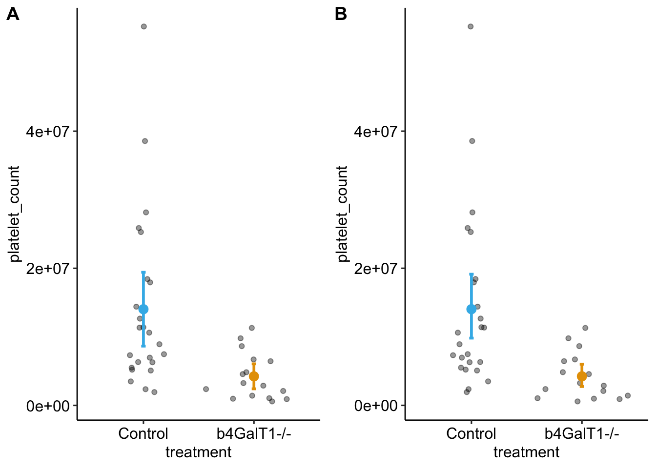
Figure 1: A. Raw 95% CI, B. Bootstrap 95% CI
Not a big difference.
Simulation
boot_sim <- function(
  mu, # mean of each level
  model = "nb", # distribution of the data, normal or nb
  theta = 1, #theta for nb
  sigma = 1, # sd of each level for normal
  beta, # coefficients of model
  n_sim = 1000, # iterations of simulation
  n_boot = 1000, # number of bootstrap resamples
  n_list = 30, # vector of sample sizes per level. Whole sim run for each n
  method = "stratified" # stratified, residual, or both
){
  k <- length(mu)
  treatment_levels <- names(mu)

  coverage_table_bca <- data.table(parameter = c(treatment_levels, "diff"))
  coverage_table_perc <- data.table(parameter = c(treatment_levels, "diff"))


  for(n in n_list){
    N <- k*n
    # vector of parameters for sampling function
    sim_mu <- rep(mu, each=n)
    sim_sigma <- rep(sigma, each=n)

    fd <- data.table(
      treatment = rep(treatment_levels, each=n)
    )
    fd[, treatment := factor(treatment, treatment_levels)]
    fd[, level := as.integer(treatment)]

    boot_ci_bca<- matrix(FALSE, nrow = n_sim, ncol=3)
    colnames(boot_ci_bca) <- c(treatment_levels, "diff")
    boot_ci_perc <- matrix(FALSE, nrow = n_sim, ncol=3)
    colnames(boot_ci_perc) <- c(treatment_levels, "diff")

    for(iter in 1:n_sim){
      if(model=="nb"){
        fd[, platelet_count := rnegbin(N, sim_mu, theta)]
      }
      if(model=="normal"){
        fd[, platelet_count := rnorm(N, sim_mu, sim_sigma)]
      }

      X_i <- cbind(model.matrix(~ treatment, data=fd), fd$platelet_count)
      boot_out <- boot(X_i,
                 strata = X_i[,2],
                 boot_diff4,
                 R = n_boot)
      # bca intervals
      ci_mean_cn <- boot.ci(boot_out, index = 1, conf=0.95, type=c("bca"))$bca[4:5]
      ci_mean_tr <- boot.ci(boot_out, index = 2, conf=0.95, type=c("bca"))$bca[4:5]
      ci_diff <- boot.ci(boot_out, index = 3, conf=0.95, type=c("bca"))$bca[4:5]
      boot_ci_bca[iter, 1] <- between(mu[1], ci_mean_cn[1], ci_mean_cn[2])
      boot_ci_bca[iter, 2] <- between(mu[2], ci_mean_tr[1], ci_mean_tr[2])
      boot_ci_bca[iter, 3] <- between(beta[2], ci_diff[1], ci_diff[2])

      # percent intervals
      ci_mean_cn <- boot.ci(boot_out, index = 1, conf=0.95, type=c("perc"))$perc[4:5]
      ci_mean_tr <- boot.ci(boot_out, index = 2, conf=0.95, type=c("perc"))$perc[4:5]
      ci_diff <- boot.ci(boot_out, index = 3, conf=0.95, type=c("perc"))$perc[4:5]
      boot_ci_perc[iter, 1] <- between(mu[1], ci_mean_cn[1], ci_mean_cn[2])
      boot_ci_perc[iter, 2] <- between(mu[2], ci_mean_tr[1], ci_mean_tr[2])
      boot_ci_perc[iter, 3] <- between(beta[2], ci_diff[1], ci_diff[2])
    }
    coverage_table_bca <- cbind(coverage_table_bca,
                               x = apply(boot_ci_bca, 2, sum)/n_sim*100)
    setnames(coverage_table_bca, "x", paste0("n=", n))

    coverage_table_perc <- cbind(coverage_table_perc,
                                 x = apply(boot_ci_perc, 2, sum)/n_sim*100)
    setnames(coverage_table_perc, "x", paste0("n=", n))
  }

  return(list(
    coverage_table_bca = coverage_table_bca,
    coverage_table_perc = coverage_table_perc
    )
  )
}
# # # # # # # # #
# This script explores "do the CIs of a x% bootstrap interval actually cover the mean x%
# of the time". The sample is from a negative binomial distribution so there is
# heterogeneity of variance.
# # # # # # # # #
set.seed(1)
n_sim <- 2000
n_boot <- 1000
n_list <- c(5, 10, 20, 40, 80)
lm_obs <- lm(platelet_count ~ treatment, data = fig1f)
lm_obs_sigma <- summary(lm_obs)$sigma
glm_obs <- glm.nb(platelet_count ~ treatment, data = fig1f)
glm_obs_fitted <- glm_obs$fitted.values
glm_obs_theta <- glm_obs$theta
mu_levels <- summary(emmeans(lm_obs, specs = "treatment"))[, "emmean"]
names(mu_levels) <- summary(emmeans(lm_obs, specs = "treatment"))[, "treatment"]
beta <- coef(lm_obs)
theta <- glm_obs_theta
sigma_raw <- fig1f_means[, SD]
names(sigma_raw) <- fig1f_means[, treatment]out_file <- "boot_ci-nb.Rds"
save_file_path <- here(output_folder, out_file)
if(run_simulation == TRUE){
boot_ci_sim_nb <- boot_sim(
mu = mu_levels, # mean of each level
model = "nb", # distribution of the data, normal or nb
theta = theta, #theta for nb
sigma = sigma_raw, # sd of each level for normal
beta = beta, # coefficients
n_sim = n_sim, # iterations of simulation
n_boot = n_boot, # number of bootstrap resamples
n_list = n_list, # vector of sample sizes per level. Whole sim run for each n
method = "stratified" # stratified, residual, or both
)
saveRDS(object = boot_ci_sim_nb, file = save_file_path)
}else{
boot_ci_sim_nb <- readRDS(save_file_path)
}
boot_ci_sim_nb$coverage_table_bca## parameter n=5 n=10 n=20 n=40 n=80
## 1: Control 81.40 87.60 92.20 93.00 93.60
## 2: b4GalT1-/- 81.35 90.20 90.75 93.05 93.80
## 3: diff 83.30 87.95 91.85 92.90 93.75boot_ci_sim_nb$coverage_table_perc## parameter n=5 n=10 n=20 n=40 n=80
## 1: Control 80.90 86.8 92.10 92.40 94.00
## 2: b4GalT1-/- 80.40 88.8 90.35 92.55 93.20
## 3: diff 83.35 88.2 92.10 93.10 93.85out_file <- "boot_ci-normal.Rds"
save_file_path <- here(output_folder, out_file)
if(run_simulation == TRUE){
boot_ci_sim_normal <- boot_sim(
mu = mu_levels, # mean of each level
model = "normal", # distribution of the data, normal or nb
theta = theta, #theta for nb
sigma = sigma_raw, # sd of each level for normal
beta = beta, # coefficients
n_sim = n_sim, # iterations of simulation
n_boot = n_boot, # number of bootstrap resamples
n_list = n_list, # vector of sample sizes per level. Whole sim run for each n
method = "stratified" # stratified, residual, or both
)
saveRDS(object = boot_ci_sim_normal, file = save_file_path)
}else{
boot_ci_sim_normal <- readRDS(save_file_path)
}
boot_ci_sim_normal$coverage_table_bca## parameter n=5 n=10 n=20 n=40 n=80
## 1: Control 82.45 89.90 93.00 94.25 94.20
## 2: b4GalT1-/- 84.05 90.85 91.25 93.75 93.65
## 3: diff 84.05 89.80 93.25 93.60 94.15boot_ci_sim_normal$coverage_table_perc## parameter n=5 n=10 n=20 n=40 n=80
## 1: Control 82.10 90.45 92.95 94.35 94.65
## 2: b4GalT1-/- 84.20 90.85 91.60 93.70 93.30
## 3: diff 84.15 90.40 93.40 93.35 94.50Summary
Coverage tables for bca
ci_nb_bca <- boot_ci_sim_nb$coverage_table_bca
ci_normal_bca <- boot_ci_sim_normal$coverage_table_bca
ycols <- colnames(ci_nb_bca)
boot_ci_table <- rbind(data.table(interval = "nb", ci_nb_bca),
                       data.table(interval = "normal", ci_normal_bca))

kable(boot_ci_table[, .SD, .SDcols = ycols],
      caption = "Coverage of 95% bca CIs",
      digits=1) %>%
  kable_styling("striped", full_width = F) %>%
  pack_rows("negative binomial", 1, 3) %>%
pack_rows("normal", 4, 6)| parameter | n=5 | n=10 | n=20 | n=40 | n=80 |
|---|---|---|---|---|---|
| negative binomial | |||||
| Control | 81.4 | 87.6 | 92.2 | 93.0 | 93.6 |
| b4GalT1-/- | 81.3 | 90.2 | 90.8 | 93.0 | 93.8 |
| diff | 83.3 | 87.9 | 91.8 | 92.9 | 93.8 |
| normal | |||||
| Control | 82.5 | 89.9 | 93.0 | 94.2 | 94.2 |
| b4GalT1-/- | 84.0 | 90.8 | 91.2 | 93.8 | 93.7 |
| diff | 84.0 | 89.8 | 93.2 | 93.6 | 94.2 |
Coverage tables for perc
ci_nb_perc <- boot_ci_sim_nb$coverage_table_perc
ci_normal_perc <- boot_ci_sim_normal$coverage_table_perc
ycols <- colnames(ci_nb_bca)
boot_ci_table <- rbind(data.table(interval = "nb", ci_nb_perc),
                       data.table(interval = "normal", ci_normal_perc))

kable(boot_ci_table[, .SD, .SDcols = ycols],
      caption = "Coverage of 95% percentile CIs",
      digits=1) %>%
  kable_styling("striped", full_width = F) %>%
  pack_rows("negative binomial", 1, 3) %>%
pack_rows("normal", 4, 6)| parameter | n=5 | n=10 | n=20 | n=40 | n=80 |
|---|---|---|---|---|---|
| negative binomial | |||||
| Control | 80.9 | 86.8 | 92.1 | 92.4 | 94.0 |
| b4GalT1-/- | 80.4 | 88.8 | 90.3 | 92.5 | 93.2 |
| diff | 83.4 | 88.2 | 92.1 | 93.1 | 93.8 |
| normal | |||||
| Control | 82.1 | 90.5 | 93.0 | 94.3 | 94.7 |
| b4GalT1-/- | 84.2 | 90.8 | 91.6 | 93.7 | 93.3 |
| diff | 84.2 | 90.4 | 93.4 | 93.3 | 94.5 |
