Analyzing longitudinal data -- a simple pre-post design
A skeletal response to a twitter question:
“ANOVA (time point x group) or ANCOVA (group with time point as a covariate) for intervention designs? Discuss.”
follow-up “Only 2 time points in this case (pre- and post-intervention), and would wanna basically answer the question of whether out of the 3 intervention groups, some improve on measure X more than others after the intervention”
Here I compare five methods using fake pre-post data, including
- lm-cov. A linear model with baseline as a covariate. This is “ANCOVA” in the ANOVA-world.
- clda. constrained longitudinal data analysis (cLDA). A linear mixed model in which the intercept is constrained to be equal (no treatment effect at time 0).
- rmanova. Repeated measures ANOVA.
- lmm. A linear mixed model version of rmanova. A difference is the rmanova will use a sphericity correction.
- two-way. Linear model with Treatment and Time and their interaction as fixed factors. Equivalent to a Two-way fixed effects ANOVA in ANOVA-world.
I use a simulation to compute Type I error rate and Power. This is far from a comprehensive simulation. Like I said, its skeletal.
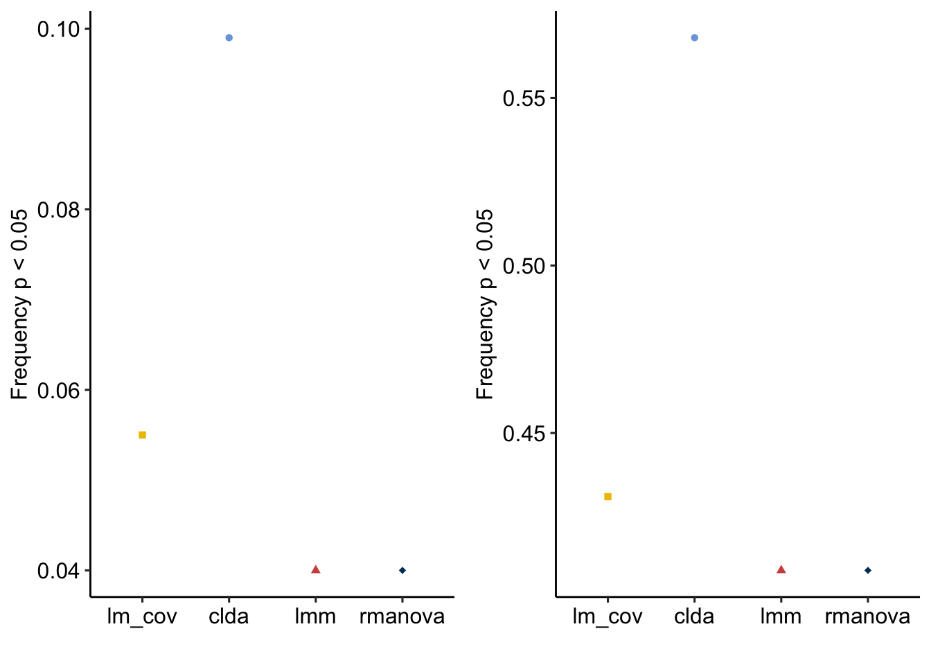
TL;DR. At the risk of concluding anything from a very skeletal simulation:
- lm-cov has best performance in since of combining control of Type I error and relative power
- smaller SE in clda comes at a cost of relatively high Type I error but increased powers. Do with this what you will.
- rmanova has smaller power than lm-cov
Not included: I didn’t save the results necessary to plot type I error conditional on baseline difference, which is well controlled by lm-cov (and clda) but not by lmm or rmanova.
libraries
library(data.table)
library(nlme)
library(emmeans)
library(afex)
library(ggpubr)
library(ggsci)
library(cowplot)
simulation functions
pre-post fake data generator
My general algorithm for creating pre-post data with a single post time point differs from how I create pre-post data with multiplee post time points.
generate_pre_post <- function(
  n = 6, # if vector then sample per group
  sigma_0 = 1, # error at time 0
  sigma_1 = 1, # error at time 1
  rho = 0.6, # correlation between time 0 and 1
  beta_0 = 10, # control mean at time 0
  beta_1 = 1, # treatment effect at time 1
  beta_2 = 5 # time effect at time 1
){

  if(length(n) == 1){n <- rep(n,2)} # set n = n for all groups
  N <- sum(n)

  fd <- data.table(
    treatment = factor(rep(c("cn", "tr"), n))
  )
  X <- model.matrix(~treatment, data=fd)

  z <- rnorm(N) # z is the common factor giving correlation at time 0 and 1. This
  # is easier for me than making glucose_1 = glucose_0 + treatment + noise
  fd[, glucose_0 := beta_0 + sqrt(rho)*z + sqrt(1 - rho)*rnorm(N, sd=sigma_0)]
  fd[, glucose_1 := beta_0 + sqrt(rho)*z*sigma_1 + sqrt(1 - rho)*rnorm(N, sd=sigma_1) +
       X[,2]*beta_1 + # add treatment effect
       beta_2 # add time effect
     ]
  fd[, change := glucose_1 - glucose_0] # change score
  fd[, id := factor(1:.N)]
  return(fd)
}
test FDG
fd <- generate_pre_post(
  n = c(10^5, 10^5),
  sigma_0 = 1,
  sigma_1 = 2,
  rho = 0.6,
  beta_0 = 10,
  beta_1 = 1
)

m1 <- lm(glucose_1 ~ treatment, data = fd)
fd[, glucose_1_cond := coef(m1)[1] + residuals(m1)]
coef(summary(m1))
## Estimate Std. Error t value Pr(>|t|)
## (Intercept) 15.0086453 0.006318270 2375.4359 0
## treatmenttr 0.9873514 0.008935383 110.4991 0cov(fd[, .SD, .SDcols=c("glucose_0", "glucose_1_cond")])## glucose_0 glucose_1_cond
## glucose_0 1.00213 1.197850
## glucose_1_cond 1.19785 3.992034cor(fd[, .SD, .SDcols=c("glucose_0", "glucose_1_cond")])## glucose_0 glucose_1_cond
## glucose_0 1.000000 0.598885
## glucose_1_cond 0.598885 1.000000coef(summary(lm(glucose_1 ~ glucose_0 + treatment, data=fd)))## Estimate Std. Error t value Pr(>|t|)
## (Intercept) 3.0529788 0.036105062 84.55819 0
## glucose_0 1.1953072 0.003574099 334.43596 0
## treatmenttr 0.9911134 0.007155790 138.50511 0fake data wide to long
wide_to_long <- function(
  dt, #data.table,
  measure_prefix = "glucose"
){
# measure _prefix is the prefix of the measurement columns that will be melted. A "_" between the prefix and a time value is assumed. So with measure vars like glucose_0, glucose_15, glucose_20, the measure prefix is "glucose"
  dt <- data.table(dt)
  dt_long <- melt(dt,
                  id.vars=c("treatment", "id"),
                  measure.vars=patterns(paste0(measure_prefix, "_")),
                  variable.name = "time",
                  value.name = measure_prefix)
  return(dt_long)
}
Fit model functions
two-way anova
two_way <- function(dt_long){
  fit <- lm(glucose ~ time*treatment, data=dt_long)
  return(fit)
}
repeated measures anova
rmanova <- function(dt_long){
  fit <- aov_4(glucose ~ time*treatment + (time|id),
               data=dt_long)
  return(fit)
}
linear model with baseline as covariate
lm_cov <- function(dt){
  fit <- lm(glucose_1 ~ glucose_0 + treatment, data = dt)
  return(fit)
}
linear mixed model
lmm <- function(dt_long){
  fit <- lme(glucose ~ time*treatment,
             random = ~1|id,
             data = dt_long,
             weights = varIdent(form= ~ 1 | time),
             correlation= corSymm(form=~ 1 | id))
  return(fit)
}
cLDA functions
Two equivalent functions for CLDA
clda-1
clda1 <- function(dt_long){
  design <- model.matrix( ~ time + treatment:time, data = dt_long)
  # remove intercept column and effect of tr at time 0
  X <- design[, -c(1, which(colnames(design) == "timeglucose_0:treatmenttr"))]
  colnames(X)[2] <- "timeglucose_1_treatmenttr"
  dt_long_x <- cbind(dt_long, X)
  form <- formula(paste0("glucose ~ ", paste(colnames(X), collapse = " + ")))
  fit <- gls(form,
            data = dt_long_x,
            weights = varIdent(form= ~ 1 | time),
            correlation= corSymm(form=~ 1| id))
  return(fit)
}
clda-2
clda2 <- function(dt_long){
  dt_clda <- copy(dt_long)
  dt_clda[, time.treatment := ifelse(time != "glucose_0" & treatment=="tr", paste0(time, ":tr"), "cont")]
  dt_clda[, time.treatment := factor(time.treatment, c("cont","glucose_1:tr"))]
  fit <- gls(glucose ~ time + time.treatment,
            data = dt_clda,
            weights = varIdent(form= ~ 1 | time),
            correlation= corSymm(form=~ 1| id))
  return(fit)
}
test functions
Some equivalents
- cLDA is equivalent estimate to the linear model with baseline covariate but has a smaller standard error.
- the two-way (fixed) ANOVA and lmm have equivalent estimates but SE is larger
- the lmm and rmanova have the same p-value (assuming sphericity)
fd <- generate_pre_post(
  n = 6,
  sigma_0 = 1,
  sigma_1 = 1,
  rho = 0.6,
  beta_0 = 10,
  beta_1 = 1
)

fd_long <- wide_to_long(fd,
                        measure_prefix = "glucose"
                        )

m1 <- lm_cov(fd)
m2 <- clda1(fd_long)
m3 <- clda2(fd_long)
m4 <- lmm(fd_long)
m5 <- two_way(fd_long)
m6 <- rmanova(fd_long)
linear model with baseline covariate
coef(summary(m1))## Estimate Std. Error t value Pr(>|t|)
## (Intercept) 9.4423880 3.3526784 2.816372 0.02016613
## glucose_0 0.5799923 0.3490826 1.661476 0.13098439
## treatmenttr 0.7087883 0.4448445 1.593340 0.14554812cLDA (both R methods)
coef(summary(m2))## Value Std.Error t-value p-value
## (Intercept) 9.6663085 0.1921116 50.316108 2.223746e-23
## timeglucose_1 5.3824640 0.3053176 17.629063 4.601669e-14
## timeglucose_1_treatmenttr 0.7087883 0.4164331 1.702046 1.035060e-01coef(summary(m3))## Value Std.Error t-value p-value
## (Intercept) 9.6663085 0.1921116 50.316108 2.223746e-23
## timeglucose_1 5.3824640 0.3053176 17.629063 4.601669e-14
## time.treatmentglucose_1:tr 0.7087883 0.4164331 1.702046 1.035060e-01two-way (fixed effect) linear model
coef(summary(m5))## Estimate Std. Error t value Pr(>|t|)
## (Intercept) 9.5630065 0.3101326 30.8352174 2.449397e-18
## timeglucose_1 5.4258517 0.4385937 12.3710192 7.923275e-11
## treatmenttr 0.2066040 0.4385937 0.4710601 6.426952e-01
## timeglucose_1:treatmenttr 0.6220131 0.6202652 1.0028179 3.279282e-01linear mixed model
coef(summary(m4))## Value Std.Error DF t-value p-value
## (Intercept) 9.5630065 0.2811776 10 34.0105547 1.142426e-11
## timeglucose_1 5.4258517 0.3172619 10 17.1021224 9.855274e-09
## treatmenttr 0.2066040 0.3976452 10 0.5195688 6.146692e-01
## timeglucose_1:treatmenttr 0.6220131 0.4486761 10 1.3863299 1.957756e-01repeated measures ANOVA
summary(m6)##
## Univariate Type III Repeated-Measures ANOVA Assuming Sphericity
##
## Sum Sq num Df Error SS den Df F value Pr(>F)
## (Intercept) 3770.9 1 8.5222 10 4424.7551 1.436e-14 ***
## treatment 1.6 1 8.5222 10 1.8863 0.1996
## time 197.5 1 3.0197 10 653.9468 1.919e-10 ***
## treatment:time 0.6 1 3.0197 10 1.9219 0.1958
## ---
## Signif. codes: 0 '***' 0.001 '**' 0.01 '*' 0.05 '.' 0.1 ' ' 1simulations
single post time point (“pre-post”)
simulate_pre_post <- function(
  niter = 1000, # number of iterations
  n = 6, # if vector then sample per group
  sigma_0 = 1, # error at time 0
  sigma_1 = 1, # error at time 1
  rho = 0.6, # correlation between time 0 and 1
  beta_0 = 10, # control mean at time 0
  beta_1 = 1, # treatment effect at time 1
  beta_2 = 5 # time effect at time 1
){

  if(length(n) == 1){n <- rep(n,2)} # set n = n for all groups
  method_list <- c("lm_cov", "clda", "lmm", "rmanova")
  prob_wide <- data.table(matrix(-9999, nrow=niter, ncol=length(method_list)))
  colnames(prob_wide) <- method_list
  for(iter in 1:niter){
    fd <- generate_pre_post(
      n = n,
      sigma_0 = sigma_0,
      sigma_1 = sigma_1,
      rho = rho,
      beta_0 = beta_0,
      beta_1 = beta_1
    )

    fd_long <- wide_to_long(fd,
                            measure_prefix = "glucose"
    )

    m1 <- lm_cov(fd)
    m2 <- clda1(fd_long)
    m3 <- clda2(fd_long)
    m4 <- lmm(fd_long)
    m5 <- two_way(fd_long)
    m6 <- rmanova(fd_long)

    prob_wide[iter, lm_cov := coef(summary(m1))["treatmenttr", "Pr(>|t|)"]]
    prob_wide[iter, clda := coef(summary(m2))["timeglucose_1_treatmenttr", "p-value"]]
    prob_wide[iter, lmm := coef(summary(m4))["timeglucose_1:treatmenttr", "p-value"]]
    prob_wide[iter, rmanova := summary(m6)$univariate.tests["treatment:time", "Pr(>F)"]]

  }

  prob <- melt(prob_wide,
               id.vars = NULL,
               measure.vars = method_list,
               variable.name = "method",
               value.name = "p_value")
  return(prob)
}
Summary statistics
p_summary <- function(prob, niter){
  prob_summary <- prob[, .(freq_lt_05 = sum(p_value < 0.05)/max(niter)),
          by = .(method)]
  return(prob_summary)
}
Plot:
plot_it <- function(prob){
  jco_pal <- pal_jco()(6)
  group_colors <- jco_pal[c(2,5,4,6)]
  group_shapes <- c(15, 16, 17,  18)

  pd <- position_dodge(0.8)
  gg1 <- ggplot(data = prob,
                aes(x=method, y=freq_lt_05, color=method, shape=method)) +
    geom_point(position = pd) +
    scale_color_manual(values = group_colors) +
    scale_shape_manual(values = group_shapes) +
    ylab("Frequency p < 0.05") +
    xlab("") +
    theme_pubr() +
    theme(legend.position="none") +
    guides(col = guide_legend(ncol = 5, byrow = FALSE)) +
    NULL
  return(gg1)
}
Type I error
# parameters of simulation
  niter = 1000 # number of iterations
  n = 6 # if vector then sample per group
  sigma_0 = 1 # error at time 0
  sigma_1 = 1 # error at time 1
  rho = 0.6 # correlation between time 0 and 1
  beta_0 = 10 # control mean at time 0
  beta_1 = 0 # treatment effect at time 1
  beta_2 = 5 # time effect at time 1

  prob_type1 <- simulate_pre_post(niter = niter,
                                  n = n,
                                  sigma_0 = sigma_0,
                                  sigma_1 = sigma_1,
                                  rho = rho,
                                  beta_0 = beta_0,
                                  beta_1 = beta_1,
                                  beta_2 = beta_2)

prob_type1_sum <- p_summary(prob_type1, niter)
Power
# parameters of simulation
  niter = 1000 # number of iterations
  n = 6 # if vector then sample per group
  sigma_0 = 1 # error at time 0
  sigma_1 = 1 # error at time 1
  rho = 0.6 # correlation between time 0 and 1
  beta_0 = 10 # control mean at time 0
  beta_1 = 1 # treatment effect at time 1
  beta_2 = 5 # time effect at time 1

  prob_power <- simulate_pre_post(niter = niter,
                              n = n,
                              sigma_0 = sigma_0,
                              sigma_1 = sigma_1,
                              rho = rho,
                              beta_0 = beta_0,
                              beta_1 = beta_1,
                              beta_2 = beta_2)

  prob_power_sum <- p_summary(prob_power, niter)
Tables
Type I error rates
table1 <- prob_type1_sum
colnames(table1)[2] <- "Type I error rate"
knitr::kable(table1)| method | Type I error rate |
|---|---|
| lm_cov | 0.055 |
| clda | 0.099 |
| lmm | 0.040 |
| rmanova | 0.040 |
Power
table2 <- prob_power_sum
colnames(table2)[2] <- "Power"
knitr::kable(table2, digits = 2)| method | Power |
|---|---|
| lm_cov | 0.43 |
| clda | 0.57 |
| lmm | 0.41 |
| rmanova | 0.41 |
Plots
gg_a <- plot_it(prob_type1_sum)
gg_b <- plot_it(prob_power_sum)
plot_grid(gg_a, gg_b, ncol=2)