
What is the range of reasonable P-values given a two standard error difference in means?
Here is the motivating quote for this post, from Andrew Gelman’s blog post “Five ways to fix statistics”
I agree with just about everything in Leek’s article except for this statement: “It’s also impractical to say that statistical metrics such as P values should not be used to make decisions. Sometimes a decision (editorial or funding, say) must be made, and clear guidelines are useful.” Yes, decisions need to be made, but to suggest that p-values be used to make editorial or funding decisions—that’s just horrible. That’s what’s landed us in the current mess. As my colleagues and I have discussed, we strongly feel that editorial and funding decisions should be based on theory, statistical evidence, and cost-benefit analyses—not on a noisy measure such as a p-value. Remember that if you’re in a setting where the true effect is two standard errors away from zero, that the p-value could easily be anywhere from 0.00006 and 1. That is, in such a setting, the 95% predictive interval for the z-score is (0, 4), which corresponds to a 95% predictive interval for the p-value of (1.0, 0.00006). That’s how noisy the p-value is. So, no, don’t use it to make editorial and funding decisions.
I’m not sure how Gelman computed these numbers, but the statement seems worthy of exploring with an R-doodle. Here is the way I’d frame the question for exploration: given a true, two SED (standard error of the difference in means) effect, what is the interval containing 95% of future \(p\)-values? Here is the R-doodle, which also explores the interval given 1, 3, and 4 SED effects.
# doodle to see 95% CI of p-value (range of p-values consistent with data) given
# a 2SE effect size (i.e. just at 0.05 for large n)
# motivating quote:
# "Remember that if you’re in a setting where the true effect is two standard errors away from zero, that the p-value could easily be anywhere from 0.00006 and 1. That is, in such a setting, the 95% predictive interval for the z-score is (0, 4), which corresponds to a 95% predictive interval for the p-value of (1.0, 0.00006). That’s how noisy the p-value is."
# source: http://andrewgelman.com/2017/11/28/five-ways-fix-statistics/
# Jeffrey Walker
# November 29, 2017

library(ggplot2)
library(data.table)
set.seed(1)
n <- 30
niter <- 5*10^3
sigma <- 1
x <- rep(c(0,1),each=n)
p <- numeric(niter)
d <- numeric(niter)
res <- data.table(NULL)
# initialize in SED units
for(sed_effect in 1:4){
  # the effect in SEM units
  se_effect <- sqrt(2*sed_effect^2) #
  # the effect in SD units
  sd_effect <- se_effect/sqrt(n)
  power <- power.t.test(n, sd_effect, sigma)$power
  y1 <- matrix(rnorm(n*niter,mean=0.0, sd=sigma), nrow=n)
  y2 <- matrix(rnorm(n*niter, mean=sd_effect, sd=sigma),nrow=n)
  for(i in 1:niter){
    p[i] <- t.test(y1[,i],y2[,i])$p.value
  }
  ci <- quantile(p, c(0.025, 0.05, 0.25, 0.5, 0.75, 0.95, 0.975))
  res <- rbind(res, data.table(n=n,
                          d.sed=sed_effect,
                          d.sem=se_effect, d.sd=round(sd_effect, 2),
                          power=round(power,2),
                          data.table(t(ci))))
}
res
## n d.sed d.sem d.sd power 2.5% 5% 25%
## 1: 30 1 1.414214 0.26 0.16 3.347471e-03 9.251045e-03 9.726431e-02
## 2: 30 2 2.828427 0.52 0.50 1.307935e-04 4.364955e-04 9.216022e-03
## 3: 30 3 4.242641 0.77 0.84 4.042272e-06 1.242138e-05 4.220133e-04
## 4: 30 4 5.656854 1.03 0.98 4.570080e-08 2.297983e-07 1.471134e-05
## 50% 75% 95% 97.5%
## 1: 0.2936458989 0.611365558 0.91934854 0.95630882
## 2: 0.0499891796 0.189903833 0.69030016 0.84298129
## 3: 0.0036464345 0.023343898 0.17671907 0.29660133
## 4: 0.0001906092 0.001769547 0.02642579 0.05377549old_names <- c('2.5%', '5%', '25%', '50%', '75%', '95%', '97.5%')
new_names <- c('lo3', 'lo2', 'lo1', 'med', 'up1', 'up2', 'up3')
setnames(res, old=old_names, new=new_names)
gg <- ggplot(data=res, aes(x=d.sed, y=med)) +
geom_linerange(aes(ymin=lo3, ymax=up3)) +
geom_linerange(aes(ymin=lo1, ymax=up1), size=4, color='darkgray') +
geom_point() +
geom_hline(yintercept=0.05, linetype='dashed') +
# geom_hline(yintercept=0.05, aes(linetype='dashed', color='darkgray'))
# geom_hline(yintercept=0.05, mapping=aes(linetype='dashed', color='red'))
labs(x='Difference in means (SED)', y='p-value') +
theme_minimal()
gg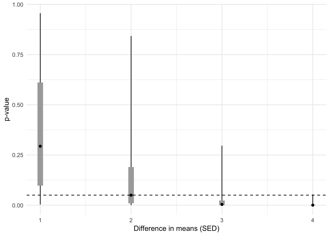
A 2 SED effect has an expected \(p\)-value near 0.05 given a reasonable sample size. My 95% interval for \(p\)-values for a 2 SED effect is (0.0001, .83), which is narrower than Gelman’s. I’m not sure we’re computing the same thing. I’ve explored the question, what is the confidence interval of the SED and \(p\)-value if the true effect, in SED units, is 2?
Regardless, the larger point remains intact. The larger point, of course, is that \(p\)-values are noisy. If an effect is just statistically significant, future \(p\)-values from the experiment would reasonably range from very small to very large (and this assumes that the only difference in future experiments is sampling variation).
