
Analyze the mean (or median) and not the max response
This is an update of Paired t-test as a special case of linear model and hierarchical model
Figure 2A of the paper Meta-omics analysis of elite athletes identifies a performance-enhancing microbe that functions via lactate metabolism uses a paired t-test to compare endurance performance in mice treated with a control microbe (Lactobacillus bulgaricus) and a test microbe (Veillonella atypica) in a cross-over design (so each mouse was treated with both bacteria). The data are in the “Supplementary Tables” Excel file, which includes the raw data for the main paper.
Endurance performance of each mouse was measured three times under each treatment level. The authors used two different analyses of the data: 1) a paired t-test between the treatments using the maximum performance over the three trials, 2) a linear mixed model with mouse ID as a random intercept (and sequence and day as covariates). A problem with the estimation of a treatment effect using the maximum response (the authors used the maximum of three endurance trials) is that the variance of the estimate of a maximum is bigger than the variance of the estimate of a mean. Consequently, the variance of the effect will be bigger, with more inflated large effects (Type M error) and more effects with the wrong sign (Type S error).
Here I repeat the analysis from the earlier post (which focussed on the paired t-test as a special case of a linear model) but add the analysis of the means and a simulation to show the effect on the variance of the estimated treatment effect.
Setup
library(ggplot2)
library(ggpubr)
library(readxl)
library(data.table)
library(lmerTest)
library(emmeans)
library(mvtnorm)

bookdown_it <- TRUE
if(bookdown_it==TRUE){
  data_path <- "../data"
  out_path <- "../output"
  source("../../../R/clean_labels.R")
}else{
  data_path <- "../content/data"
  out_path <- "../content/output"
  source("../../R/clean_labels.R")
}
Import
folder <- "Data from Meta-omics analysis of elite athletes identifies a performance-enhancing microbe that functions via lactate metabolism"
file_i <- "41591_2019_485_MOESM2_ESM.xlsx"
file_path <- paste(data_path, folder, file_i, sep="/")
sheet_i <- "ST3 Veillonella run times"
range_vec <- c("a5:d21", "f5:i21", "a24:d40", "f24:i40")
fig2a.orig <- data.table(NULL)
poop <- c("Lb", "Va")
for(week_i in 1:4){
  range_i <- range_vec[week_i]
  if(week_i %in% c(1, 3)){
    treatment <- rep(c(poop[1], poop[2]), each=8)
  }else{
    treatment <- rep(c(poop[2], poop[1]), each=8)
  }
  fig2a.orig <- rbind(fig2a.orig, data.table(week=week_i, treatment=treatment, data.table(
    read_excel(file_path, sheet=sheet_i, range=range_i))))
}

# clean column names
setnames(fig2a.orig, old="...1", new="ID")
setnames(fig2a.orig, old=colnames(fig2a.orig), new=clean_label(colnames(fig2a.orig)))

# add treatment sequence
fig2a.orig[, sequence:=rep(rep(rep(c("LLLVVV", "VVVLLL"), each=8), 2), 2)]

# wide to long
fig2a <- melt(fig2a.orig, id.vars=c("week", "ID", "treatment", "sequence"),
              variable.name="day",
              value.name="time")
Because of the cross-over design, the ID is not in order within each level of treatment. Make a wide data table with new treatment columns matched by ID.
# get max for each week x ID x treatment combo
fig2a.max <- fig2a[, .(time_max=max(time)), by=.(week, ID, treatment)]

# match the two treatments applied to each ID
va <- fig2a.max[treatment=="Va", ]
lb <- fig2a.max[treatment=="Lb", ]
fig2a_wide <- merge(va, lb, by="ID")
Comparison
paired t-test
# paired t
res.t <- t.test(fig2a_wide[, time_max.x], fig2a_wide[, time_max.y], paired=TRUE)
res.t
##
## Paired t-test
##
## data: fig2a_wide[, time_max.x] and fig2a_wide[, time_max.y]
## t = 2.4117, df = 31, p-value = 0.02199
## alternative hypothesis: true difference in means is not equal to 0
## 95 percent confidence interval:
## 20.47859 244.89641
## sample estimates:
## mean of the differences
## 132.6875linear model
# as a linear model
y <- fig2a_wide[, time_max.x] - fig2a_wide[, time_max.y] # Va - Lb
res.lm <- lm(y ~ 1)
coef(summary(res.lm))
## Estimate Std. Error t value Pr(>|t|)
## (Intercept) 132.6875 55.01749 2.411733 0.02198912hierarchical (linear mixed) model with random intercept
# as multi-level model with random intercept
res.lmer <- lmer(time_max ~ treatment + (1|ID), data=fig2a.max)
coef(summary(res.lmer))
## Estimate Std. Error df t value Pr(>|t|)
## (Intercept) 1023.7187 43.37421 59.71689 23.602014 5.703668e-32
## treatmentVa 132.6875 55.01752 30.99995 2.411732 2.198920e-02Re-analysis – What about the mean and not max response?
Paired t-test of means
# t test
# get mean for each week x ID x treatment combo
fig2a.mean <- fig2a[, .(time_mean=mean(time)), by=.(week, ID, treatment)]
va <- fig2a.mean[treatment=="Va", ]
lb <- fig2a.mean[treatment=="Lb", ]
fig2a_wide <- merge(va, lb, by="ID")
res.t <- t.test(fig2a_wide[, time_mean.x], fig2a_wide[, time_mean.y], paired=TRUE)
res.t
##
## Paired t-test
##
## data: fig2a_wide[, time_mean.x] and fig2a_wide[, time_mean.y]
## t = 1.7521, df = 31, p-value = 0.08964
## alternative hypothesis: true difference in means is not equal to 0
## 95 percent confidence interval:
## -12.38639 163.40722
## sample estimates:
## mean of the differences
## 75.51042The p-value of the t-test using max performance was 0.02 and that using mean performance is 0.09. These aren’t too different (do not be distracted by the fact that they fall on opposite sides of 0.05) but neither inspires much confidence that the effect will reproduce.
Hierarchical model
# hierarchical model
res2.lmer <- lmer(time ~ treatment + (1|ID), data=fig2a)
coef(summary(res2.lmer))
## Estimate Std. Error df t value Pr(>|t|)
## (Intercept) 848.25000 32.09252 65.82282 26.431394 9.129879e-37
## treatmentVa 75.51042 36.83330 159.00005 2.050059 4.200108e-02The p-value is 0.04, which differs from that for the t-test because this model is fit to all the data and not just the mean values.
Simulation
A simulation of Type I, II, M and S error that arises when estimating the treatment effect from differences in the maximum response.
set.seed(1)
do_sim <- FALSE
if(do_sim==TRUE){
  n <- 32
  p <- 3 # number of trials
  mu <- coef(summary(res2.lmer))[1, "Estimate"]
  beta <- coef(summary(res2.lmer))[2, "Estimate"]
  sigma <- as.data.frame(VarCorr(res2.lmer))[2, "sdcor"]
  sigma_id <- as.data.frame(VarCorr(res2.lmer))[1, "sdcor"]
  icc <- sigma_id^2/(sigma_id^2 + sigma^2)
  icov <- matrix(icc*sigma_id^2, nrow=3, ncol=3) # covariance
  diag(icov) <- sigma^2

  niter <- 5000
  b.max <- numeric(niter)
  b.mean <- numeric(niter)
  b.lmer <- numeric(niter)
  p.max <- numeric(niter)
  p.mean <- numeric(niter)
  p.lmer <- numeric(niter)
  mean.max <- numeric(niter)
  mean.mean <- numeric(niter)
  sim_table <- data.table(NULL)

  mu_i <- rnorm(n, mean=mu, sd=sigma_id) # true performance in treatment A

  for(b1 in c(0, beta)){
    for(iter in 1:niter){
      # performance_A <- matrix(rnorm(n*p, mean=mu, sd=sqrt(sigma^2 + sigma_id^2)), nrow=n)
      # performance_B <- matrix(rnorm(n*p, mean=mu, sd=sqrt(sigma^2 + sigma_id^2)), nrow=n) + b1

      # performance_A <- matrix(rnorm(n*p, mean=mu_i, sd=sigma), nrow=n)
      # performance_B <- matrix(rnorm(n*p, mean=mu_i, sd=sigma), nrow=n) + b1
      #
      performance_A <- rmvnorm(n, mean=rep(0, p), sigma=icov) + matrix(mu_i, nrow=n, ncol=p)
      performance_B <- rmvnorm(n, mean=rep(0, p), sigma=icov) + matrix(mu_i, nrow=n, ncol=p) + b1

      # t test of max
      A <- apply(performance_A, 1, max)
      B <- apply(performance_B, 1, max)
      mean.max[iter] <- mean(A)
      t_res <- t.test(B, A, paired=TRUE)
      b.max[iter] <- t_res$estimate
      p.max[iter] <- t_res$p.value

      # t test of mean
      A <- apply(performance_A, 1, mean)
      B <- apply(performance_B, 1, mean)
      mean.mean[iter] <- mean(A)
      t_res <- t.test(B, A, paired=TRUE)
      b.mean[iter] <- t_res$estimate
      p.mean[iter] <- t_res$p.value

      # # hierarchical model
      performance <- rbind(data.table(treatment="A", ID=1:n, performance_A),
                           data.table(treatment="B", ID=1:n, performance_B))
      performance <- melt(performance, id.vars=c("ID", "treatment"),
                          variable.name="day",
                          value.name="time")
      sim.lmer <- lmer(time ~ treatment + (1|ID), data=performance)
      b.lmer[iter] <- coef(summary(sim.lmer))[2, "Estimate"]
      p.lmer[iter] <- coef(summary(sim.lmer))[2, "Pr(>|t|)"]
    }
    sim_table <- rbind(sim_table, data.table(effect = b1,
                                             b_max = b.max,
                                             b_mean = b.mean,
                                             b_lmer = b.lmer,
                                             p_max = p.max,
                                             p_mean = p.mean,
                                             p_lmer = p.lmer,
                                             mean_max = mean.max,
                                             mean_mean = mean.mean))
  }
  write.table(sim_table, paste(out_path,"june-25-2019.txt",sep="/"),
              row.names = FALSE, quote=FALSE, sep="\t")
}else{ # read file from simulation
  sim_table <- fread(paste(out_path,"june-25-2019.txt",sep="/"))
}
The SD among times using max performance is 34.1 and using mean performance is 26.5.
The increased variance of estimating the treatment using the maximum performance decreases power. The hierarchical model, which uses all the data, has the most power (at some cost to Type I?).
niter <- nrow(sim_table)/2
error_table <- data.table(Method=c("max", "mean", "lmm"),
                     "Type 1" = c(sum(sim_table[effect==0, p_max < 0.05])/niter,
                     sum(sim_table[effect==0, p_mean < 0.05])/niter,
                     sum(sim_table[effect==0, p_lmer < 0.05])/niter),
                     "Power" = c(sum(sim_table[effect!=0, p_max < 0.05])/niter,
                     sum(sim_table[effect!=0, p_mean < 0.05])/niter,
                     sum(sim_table[effect!=0, p_lmer < 0.05])/niter))
knitr::kable(error_table, digits=c(NA, 3, 3))| Method | Type 1 | Power |
|---|---|---|
| max | 0.050 | 0.323 |
| mean | 0.048 | 0.489 |
| lmm | 0.057 | 0.530 |
Type S and M error can be seen by looking at the distribution of effects (more inflated effects, and more sign effects)
sim_table_long <- melt(sim_table, id.vars=c("effect"),
                       measure.vars=c("b_max", "b_mean", "b_lmer"),
                       variable.name="method",
                       value.name="estimate"
                       )
gg <- ggplot(data=sim_table_long, aes(x=method, y=estimate)) +
  geom_boxplot() +
  facet_grid(.~effect, labeller = "label_both") +
  NULL
gg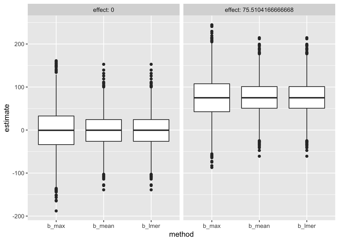
Run through a statistical significance filter, the mean effects, of those that are significant, estimated using the max response, the mean response, and a hierarchical model, are:
p_table_long <- melt(sim_table, id.vars=c("effect"),
                       measure.vars=c("p_max", "p_mean", "p_lmer"),
                       variable.name="method",
                       value.name="p"
                       )
knitr::kable(sim_table_long[effect!=0 & estimate > 0 & p_table_long[, p] < 0.05,
.(effect=mean(estimate)), by=method], digits=c(NA, 1))| method | effect |
|---|---|
| b_max | 126.8 |
| b_mean | 105.4 |
| b_lmer | 103.7 |
which is inflated for all three (the true effect is 75.5) but most inflated using maximum performance.
