
Is the power to test an interaction effect less than that for a main effect?
I was googling around and somehow landed on a page that stated “When effect coding is used, statistical power is the same for all regression coefficients of the same size, whether they correspond to main effects or interactions, and irrespective of the order of the interaction”. Really? How could this be? The p-value for an interaction effect is the same regardless of dummy or effects coding, and, with dummy coding (R’s default), the power of the interaction effect is less than that of the coefficients for the main factors when they have the same magnitude, so my intuition said this statement must be wrong.
TL;DR It depends on how one defines “main” effect or how one parameterizes the model. If “main” effect is defined as the coefficient of a factor from a dummy-coded model (that is, the added effect due to treatment), the power to test the interaction is less than that for a main effect if the two effects have the same magnitude. But, if defined as the coefficient of a factor from an effects-coded model, the power to test the interaction is the same as that for the main effect, if the two have equal magnitude (just as the source states). That said, an interaction effect using effects coding seems like a completely mathematical construct and not something “real”…or maybe I’m just re-ifying a dummy-coded interaction effect.
Updated I read this when it was posted but forgot about it when I started this doodle: Andrew Gelman has a highly relevant blog post You need 16 times the sample size to estimate an interaction than to estimate a main effect that is really minimal in that it focusses entirely on the standard error. Gelman effectively used a -0.5, +0.5 contrast coding but added an update with -1, +1 (effects) coding. This coding is interesting and explored below.
Some definitions
Consider a \(2 \times 2\) factorial experiment, factor A has two levels (-, +), factor B has two levels (-, +), and the means of the combinations are
| B- | B+ | |
|---|---|---|
| A- | \(\mu_{11}\) | \(\mu_{12}\) |
| A+ | \(\mu_{21}\) | \(\mu_{22}\) |
then the coefficients are
| dummy | effects | |
|---|---|---|
| intercept | \(\mu_{11}\) | \((\mu_{11} + \mu_{21} + \mu_{12} + \mu_{22})/4\) |
| \(\beta_A\) | \(\mu_{21} - \mu_{11}\) | \(-((\mu_{21} - \mu_{11}) + (\mu_{22} - \mu_{12}))/2\) |
| \(\beta_B\) | \(\mu_{12} - \mu_{11}\) | \(-((\mu_{12} - \mu_{11}) + (\mu_{22} - \mu_{21}))/2\) |
| \(\beta_{AB}\) | \(\mu_{22} - (intercept + \beta_A + \beta_B)\) | \(\mu_{11} - (intercept + \beta_A + \beta_B)\) |
Or, in words, with dummy coding
- the intercept is the mean of the group with no added treatment in either A or B (it is the control)
- \(\beta_A\) is the effect of treatment A when no treatment has been added to B
- \(\beta_B\) is the effect of treatment B when no treatment has been added to A
- \(\beta_{AB}\) is “the leftovers”, that is, the non-additive effect. It is the difference between the mean of the group in which both A and B treatments are added and the expected mean of this group if A and B act additively (that is, if we add the A and B effects).
and, with effects coding
- the intercept is the grand mean
- \(\beta_A\) is -1 times half the average of the simple effects of A, where the simple effects of A are the effects of A within each level of B
- \(\beta_B\) is -1 times half the average of the simple effects of B, where the simple effects of B are the effects of B within each level of A
- \(\beta_{AB}\) is “the leftovers”, that is, the non-additive effect, it is the difference between the mean of the group with the “control” levels of A and B and the expected mean of this group if A and B act additively (The magnitude is the difference between any mean and the additive effect but the sign of the difference depends on which group).
\(\beta_A\) and \(\beta_B\) are often called the “main” effects and \(\beta_{AB}\) the “interaction” effect. The table shows why these names are ambiguous. To avoid this ambiguity, it would be better to refer to \(\beta_A\) and \(\beta_B\) in dummy-coding as “simple” effects. There are as many simple effects as levels of the other factor. And the simple effect coefficient for the dummy-coded model depends on which level of the factor is set as the “reference”.
Finally, note that while the interaction effect in dummy and effects coding have the same verbal meaning, they have a different numerical value because the “main” effect differs between the codings.
Visualizing interaction effects
Given a set of means
| B- | B+ | |
|---|---|---|
| A- | \(\mu_{11}=0\) | \(\mu_{12}=0.5\) |
| A+ | \(\mu_{21}=0.5\) | \(\mu_{22}=1.5\) |
To generate these data using dummy coding, the coefficients are (0, .5, .5, .5) and using effects coding the coefficients are (.625, -.375, -.375, .125). The interaction coefficients using the two parameterization is visualized with arrows…
dummy_2_effects <- function(b){

  b3 <- numeric(4)
  b3[1] <- (b[1] + (b[1] + b[2]) + (b[1] + b[3]) + (b[1] + b[2] + b[3] + b[4]))/4
  b3[2] <- -(b[2] + (b[2] + b[4]))/2/2
  b3[3] <- -(b[3] + (b[3] + b[4]))/2/2
  b3[4] <- b[1] - (b3[1] + b3[2] + b3[3])
  return(b3)
}

con3 <- list(CO2=contr.sum, Temp=contr.sum) # change the contrasts coding for the model matrix
n <- 1
a_levels <- c("current", "high")
b_levels <- c("current", "high")
N <- n * length(a_levels) * length(b_levels)
x_cat <- data.table(expand.grid(CO2=a_levels, Temp=b_levels))
x_cat <- x_cat[rep(seq_len(nrow(x_cat)), each=n)]
X1 <- model.matrix(~CO2*Temp, data=x_cat)
X3 <- model.matrix(~CO2*Temp, contrasts=con3, data=x_cat)

beta1 <- c(0, 0.5, 0.5, 0.5)
beta3 <- dummy_2_effects(beta1)

y1 <- (X1%*%beta1)[,1]
y1.a <- (X1[,1:3]%*%beta1[1:3])[,1]
y3 <- (X3%*%beta3)[,1] # should = y1
y3.a <- (X3[,1:3]%*%beta3[1:3])[,1]

fd <- cbind(x_cat, y1.a=y1.a, y1=y1, y3=y3, y3.a=y3.a)

gg.dummy <- ggplot(data=fd, aes(x=CO2, y=y1.a, shape=Temp)) +
  geom_point(size=3, color="red") +
  geom_point(aes(y=y1, shape=Temp), size=3, color="black") +
  geom_segment(aes(x=2, y=fd[4, y1.a], xend=2, yend=fd[4, y1]-0.02), arrow=arrow(length = unit(0.2,"cm"))) +
  scale_y_continuous(limits=c(-0.15, 1.75)) +
  ylab("y") +
  theme(legend.position="bottom") +
  NULL

gg.effects <- ggplot(data=fd, aes(x=CO2, y=y3.a, shape=Temp)) +
  geom_point(size=3, color="red") +
  geom_point(aes(y=y3), size=3, color="black") +
  geom_segment(aes(x=1, y=fd[1, y3.a], xend=1, yend=fd[1, y3]-0.02), arrow=arrow(length = unit(0.2,"cm"))) +
  geom_segment(aes(x=2, y=fd[2, y3.a], xend=2, yend=fd[2, y3]+0.02), arrow=arrow(length = unit(0.2,"cm"))) +
  geom_segment(aes(x=1, y=fd[3, y3.a], xend=1, yend=fd[3, y3]+0.02), arrow=arrow(length = unit(0.2,"cm"))) +
  geom_segment(aes(x=2, y=fd[4, y3.a], xend=2, yend=fd[4, y3]-0.02), arrow=arrow(length = unit(0.2,"cm"))) +
  scale_y_continuous(limits=c(-0.15, 1.75)) +
  ylab("y") +
  theme(legend.position="bottom") +
  NULL

plot_grid(gg.dummy, gg.effects, ncol=2, labels=c("A. Dummy coding", "B. Effects coding"))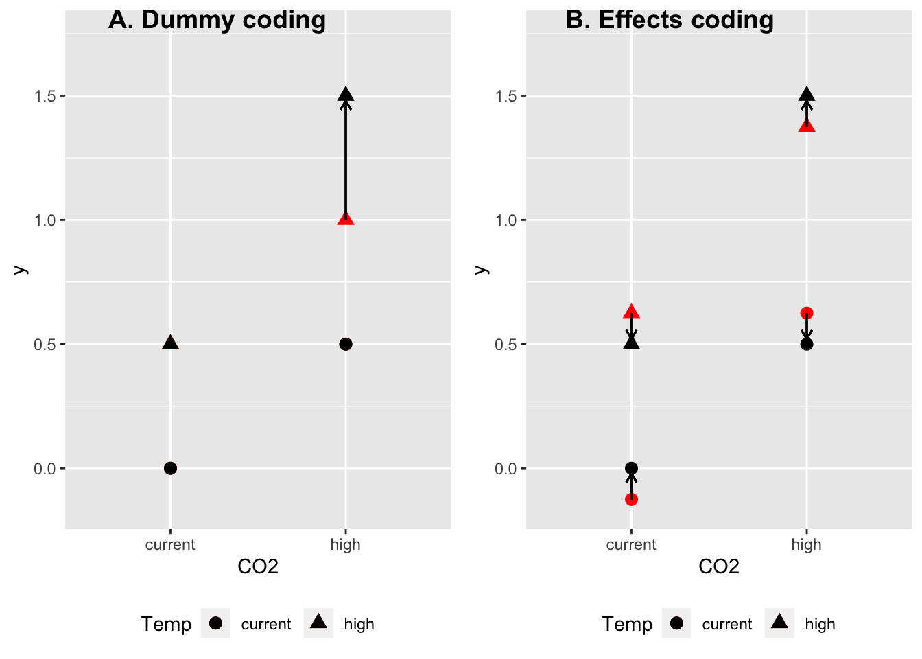
Figure 1: illustration of interaction effect computed using A) dummy coding and B) effects coding. Black dots are the true means. Red dots are the expected means given only additive effects. The interaction effect is ‘what is left’ to get from the expectation using only additive effects to the true mean. With a dummy coded model, there is only one interaction effect for the 2 x 2 design. With an effects coded model, there are four interaction effects – all have the same magnitude but the sign varies by group.
In the dummy coded parameterization (A), if we interpret the coefficients as “effects” then the interaction effect is the same as the “main” effects. The interaction effect is shown by the single arrow and it is applied to \(\mu_{22}\) only
In the effects coded parameterization (B), the means are precisely the same as in (A), and if we interpret the coefficients as the effects, then the interaction effect is 1/3 the magnitude of the main effects. Again, these are the same means as in (A). The difference with A is that the interaction is applied to all four means – there isn’t “an” interaction effect but four. And note that the sum of the four interaction effects equals the sum of the one effect in (A).
So, how we think about the “magnitude” of the interaction depends on how we parameterize the model or how we think about the effects. If we think of the non-reference (“treated”) levels of Factors A and B (CO2 and Temp) as “adding” something to the control’s value, then, thinking about an interaction using dummy coding makes sense. But if we think about the levels of a factor as simply being variable about a mean, then the interaction using effects coding makes sense, though I might be inclined to model this using a hierarchical rather than fixed effects model.
What about Gelman coded contrasts?
Andrew Gelman uses a (-0.5, .5) contrast instead of the (1, -1) contrast used in effects coding. The consequence of this is that a main effect coefficient is the average treatment effect (the difference averaged over each level of the other factor) instead of half the average treatment effect. And the interaction is a “difference in differences” (\((\mu_{22}-\mu_{12}) - (\mu_{21}-\mu_{11})\)) but is not “what is leftover” as in both dummy coding and effects coding. The interaction coefficient has the same magnitude as that using dummy coding but unlike in dummy coding, the interaction effect is smaller than the main effect coefficients because the main effect coefficients are the average of the small (0.5) and big (1.5) simple effects.
And, unlike the dummy coded interaction coefficient and the effects coded interaction coefficient, it’s hard to know how to “visualize” it, since it’s magnitude is not what is “left over”. That is, the coefficients from the Gelman coded model don’t just add up to get the means as in dummy coding and treatment coding but instead, the coefficients in the sum have to be weighted by 0.5 for the main effects and 0.25 for the interaction effect. So I’m not even sure how to visualize this. Below, I’ve illustrated the Gelman-coded interaction effect as what is left-over, using the weighted sum to get the expectation of the means using only additive effects, and it looks exactly like the illustration of the interaction effect using effects coding, but the length of each arrow is the magnitude of the interaction coefficient using effects coding but only 1/4 the magnitude of the interaction coefficient using Gelman coding.
dummy_2_gelman <- function(b){

  b3 <- numeric(4)
  b3[1] <- (b[1] + (b[1] + b[2]) + (b[1] + b[3]) + (b[1] + b[2] + b[3] + b[4]))/4
  b3[2] <- (b[2] + (b[2] + b[4]))/2
  b3[3] <- (b[3] + (b[3] + b[4]))/2
  b3[4] <- b[1] - (-b3[1]/2 - b3[2]/2 + b3[3]/4)
  return(b3)
}

beta.g <- dummy_2_gelman(beta1)
con.gelman <- list(CO2=c(-0.5, .5), Temp=c(-0.5, .5)) # change the contrasts coding for the model matrix
Xg <- model.matrix(~CO2*Temp, contrasts=con.gelman, data=x_cat)

yg <- (Xg%*%beta.g)[,1] # should = y1
yg.a <- (Xg[,1:3]%*%beta.g[1:3])[,1]

fd <- cbind(fd, yg=yg, yg.a=yg.a)

gg.gelman <- ggplot(data=fd, aes(x=CO2, y=yg.a, shape=Temp)) +
  geom_point(size=3, color="red") +
  geom_point(aes(y=yg), size=3, color="black") +
  geom_segment(aes(x=1, y=fd[1, yg.a], xend=1, yend=fd[1, yg]-0.02), arrow=arrow(length = unit(0.2,"cm"))) +
  geom_segment(aes(x=2, y=fd[2, yg.a], xend=2, yend=fd[2, yg]+0.02), arrow=arrow(length = unit(0.2,"cm"))) +
  geom_segment(aes(x=1, y=fd[3, yg.a], xend=1, yend=fd[3, yg]+0.02), arrow=arrow(length = unit(0.2,"cm"))) +
  geom_segment(aes(x=2, y=fd[4, yg.a], xend=2, yend=fd[4, yg]-0.02), arrow=arrow(length = unit(0.2,"cm"))) +
  scale_y_continuous(limits=c(-0.15, 1.75)) +
  ylab("y") +
  theme(legend.position="bottom") +
  NULL

plot_grid(gg.effects, gg.gelman, ncol=2, labels=c("A. Effects coding", "B. Gelman coding"))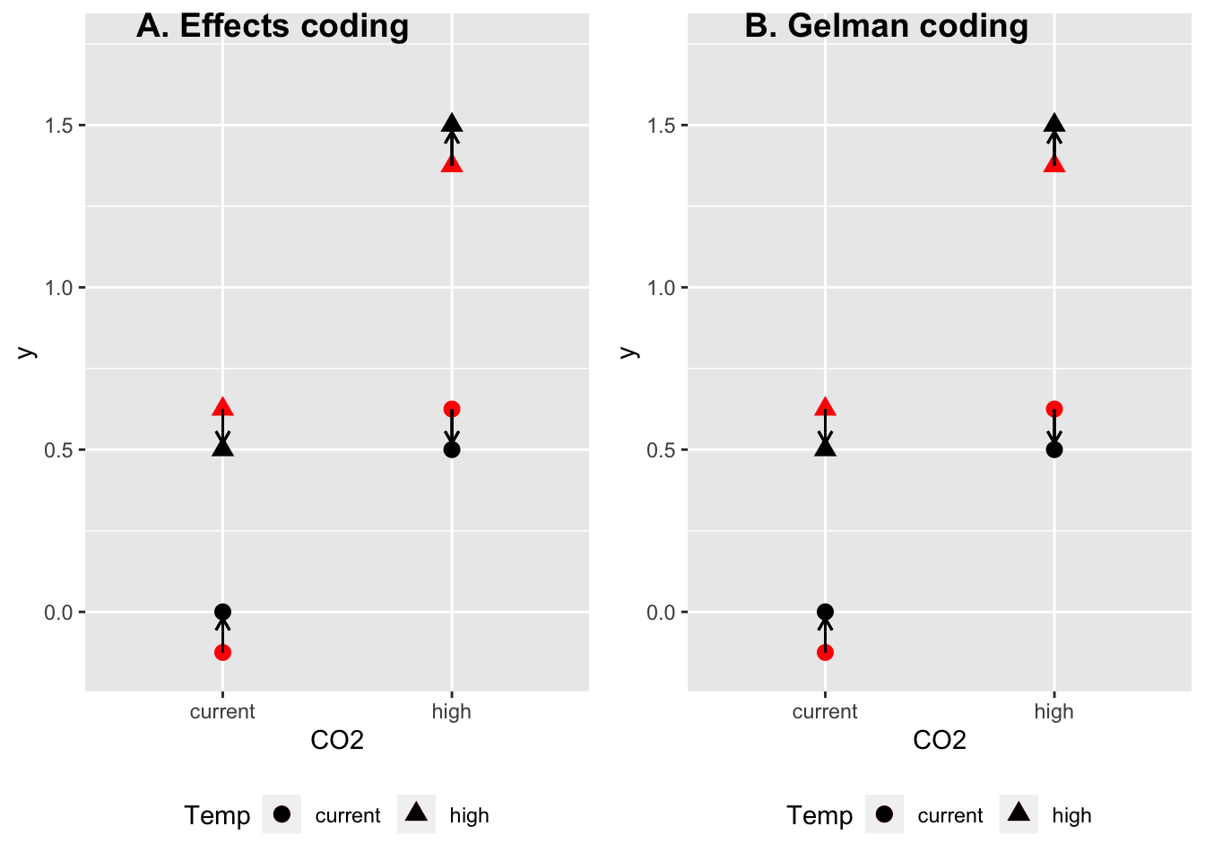
The interaction effect computed using treatment (dummy) coding does not equal the interaction effect computed using effect coding.
Many researchers look only at ANOVA tables (and not a coefficients table) where the p-value of the interaction term is the same regardless of the sum-of-squares computation (sequential SS using dummy coding or Type III SS using effects coding). By focussing on the p-value, it’s easy to miss that the interaction coefficient and SE differ between the two types of coding.
Script to compare dummy and effect coding with small n to show different estimates of interaction coefficient but same p-value.
set.seed(1)
# parameters to generate data using dummy coding generating model
beta1 <- c(0, 0.5, 0.5, 0.5)
a_levels <- c("-", "+")
b_levels <- c("-", "+")

n <- 10
N <- n * length(a_levels) * length(b_levels)
x_cat <- data.table(expand.grid(A=a_levels, B=b_levels))
x_cat <- x_cat[rep(seq_len(nrow(x_cat)), each=n)]
X <- model.matrix(~A*B, data=x_cat)
y <- (X%*%beta1)[,1] + rnorm(N)
m1 <- lm(y ~ A*B, data=x_cat)
con3 <- list(A=contr.sum, B=contr.sum) # change the contrasts coding for the model matrix
m2 <- lm(y ~ A*B, contrasts=con3, data=x_cat)
The generating coefficients (using a dummy-coding generating model) are 0, 0.5, 0.5, 0.5
The coefficients of the dummy-coded model fit to the data are:
knitr::kable(coef(summary(m1)), digits=c(2,4,1,4))| Estimate | Std. Error | t value | Pr(>|t|) | |
|---|---|---|---|---|
| (Intercept) | 0.13 | 0.2881 | 0.5 | 0.6491 |
| A+ | 0.62 | 0.4074 | 1.5 | 0.1389 |
| B+ | 0.23 | 0.4074 | 0.6 | 0.5691 |
| A+:B+ | 0.64 | 0.5762 | 1.1 | 0.2757 |
And the coefficients of the effects-coded model fit to the same data are:
knitr::kable(coef(summary(m2)), digits=c(2,4,1,4))| Estimate | Std. Error | t value | Pr(>|t|) | |
|---|---|---|---|---|
| (Intercept) | 0.72 | 0.1441 | 5.0 | 0.0000 |
| A1 | -0.47 | 0.1441 | -3.2 | 0.0025 |
| B1 | -0.28 | 0.1441 | -1.9 | 0.0629 |
| A1:B1 | 0.16 | 0.1441 | 1.1 | 0.2757 |
Note that
- the “main” effect coefficients in the two tables are not estimating the same thing. In the dummy coded table, the coefficients are not “main” effect coefficients but “simple” effect coefficients. They are the difference between the two levels of one factor when the other factor is set to it’s reference level. In the effects coded table, the coefficients are “main” effect coefficients – these coefficients are equal to half the average of the two simple effects of one factor (each simple effect is within one level of the other factor).
- The interaction coefficient in the two tables is not estimating the same thing. This is less obvious, since the p-value is the same.
- the SEs differ among the in the table from the dummy coded fit but are the same in the table from the effect coded fit. The SE in the dummy coded fit is due to the number of means computed to estimate the effect: the intercept is a function of one mean, the simple effect coefficients (Aa and Bb) are functions of two means, and the interaction is a function of 4 means. Consequently, there is less power to test the main coefficients and even less to test the inrteraction coefficient. By contrast in the effect coded fit, all four coefficients are function of all four means, so all four coefficients have the same SE. That is, there is equal power to estimate the interaction as a main effect.
Script to compare dummy and effect coding using data with big n to show different models really are estimating different coefficients.
set.seed(2)
# parameters to generate data using dummy coding generating model
beta1 <- c(0, 1, 1, 1)
a_levels <- c("-", "+")
b_levels <- c("-", "+")
n <- 10^5
N <- n * length(a_levels) * length(b_levels)
x_cat <- data.table(expand.grid(A=a_levels, B=b_levels))
x_cat <- x_cat[rep(seq_len(nrow(x_cat)), each=n)]
X <- model.matrix(~A*B, data=x_cat)
y <- (X%*%beta1)[,1] + rnorm(N)
m1 <- lm(y ~ A*B, data=x_cat)
con3 <- list(A=contr.sum, B=contr.sum) # change the contrasts coding for the model matrix
m2 <- lm(y ~ A*B, contrasts=con3, data=x_cat)
The generating coefficients (using a dummy-coding generating model) are 0, 1, 1, 1
The coefficients of the dummy-coded model fit to the data are:
knitr::kable(coef(summary(m1)), digits=c(2,4,1,4))| Estimate | Std. Error | t value | Pr(>|t|) | |
|---|---|---|---|---|
| (Intercept) | 0.00 | 0.0032 | 1.0 | 0.3303 |
| A+ | 1.00 | 0.0045 | 223.3 | 0.0000 |
| B+ | 0.99 | 0.0045 | 221.6 | 0.0000 |
| A+:B+ | 1.01 | 0.0063 | 159.9 | 0.0000 |
And the coefficients of the effects-coded model fit to the same data are:
knitr::kable(coef(summary(m2)), digits=c(2,4,1,4))| Estimate | Std. Error | t value | Pr(>|t|) | |
|---|---|---|---|---|
| (Intercept) | 1.25 | 0.0016 | 791.0 | 0 |
| A1 | -0.75 | 0.0016 | -475.6 | 0 |
| B1 | -0.75 | 0.0016 | -473.3 | 0 |
| A1:B1 | 0.25 | 0.0016 | 159.9 | 0 |
Note that the coefficients generating the data using dummy coding are the same for the simple (Aa and Bb) effects, and for the interaction effect. The model fit using dummy coding recovers these, so the interaction coefficient is the same as the Aa or Bb coefficient. By contrast the interaction coefficient estimated using effects coding is 1/3 the magnitude of the main effect (A1 or B1) coefficients.
The above is the explainer for the claim that there is less power to estimate an interaction effect. There are two ways to think about this:
- Fitting a dummy coded model to the data, the SE of the interaction effect is \(2\sqrt(2)\) times the SE of the simple effects, so for coefficients of the same magnitude, there is less power. Also remember that the simple effect coefficients are not “main” effects! So there is less power to estimate an interaction effect than a simple effect of the same magnitude, but this doesn’t address the motivating point.
- Fitting an effects coded model to the data, but thinking about the interaction effect as if it were generated using a dummy coded generating model, the interaction effect is 1/3 the size of the main effect coefficients, so there is less power because this magnitude difference – the SEs of the coefficients are the same, which means that if the interaction and main effects had the same magnitude, they would have the same power.
A simulation to show that the power to test an interaction effect equals that to test a main effect if they have the same magnitude.
niter <- 10*10^3
con3 <- list(A=contr.sum, B=contr.sum) # change the contrasts coding for the model matrix
con.gelman <- list(A=c(-0.5, .5), B=c(-0.5, .5)) # change the contrasts coding for the model matrix

# parameters for data generated using dummy coding
# interaction and simple effects equal if using dummy coded model
beta1 <- c(0, 0.5, 0.5, 0.5)
Beta1 <- matrix(beta1, nrow=4, ncol=niter)

# parameters for data generated using effects coding -
# interaction and main effects equal if fit using effects coded model
beta3 <- c(0, 0.5, 0.5, 0.5)
Beta3 <- matrix(beta3, nrow=4, ncol=niter)

a_levels <- c("-", "+")
b_levels <- c("-", "+")
n <- 10
N <- n * length(a_levels) * length(b_levels)
x_cat <- data.table(expand.grid(A=a_levels, B=b_levels))
x_cat <- x_cat[rep(seq_len(nrow(x_cat)), each=n)]
X1 <- model.matrix(~A*B, data=x_cat)
X3 <- model.matrix(~A*B, contrasts=con3, data=x_cat)

fd1 <- X1%*%Beta1 + matrix(rnorm(niter*N), nrow=N, ncol=niter)
fd3 <- X3%*%Beta3 + matrix(rnorm(niter*N), nrow=N, ncol=niter)

p_labels <- c("A1", "AB1", "A3", "AB3")
p <- matrix(nrow=niter, ncol=length(p_labels))
colnames(p) <- p_labels

j <- 1

for(j in 1:niter){
  # dummy coding
  m1 <- lm(fd1[,j] ~ A*B, data=x_cat)
  m3 <- lm(fd3[,j] ~ A*B, contrasts=con3, data=x_cat)
  p[j, 1:2] <- coef(summary(m1))[c(2,4), "Pr(>|t|)"]
  p[j, 3:4] <- coef(summary(m3))[c(2,4), "Pr(>|t|)"]
}

power_res <- apply(p, 2, function(x) sum(x<0.05)/niter)
power_table <- data.frame(power=power_res)
row.names(power_table) <- c("dummy: simple A",
                            "dummy: interaction",
                             "effects: main A",
                            "effects: interaction"
                           )
kable(power_table)| power | |
|---|---|
| dummy: simple A | 0.1982 |
| dummy: interaction | 0.1218 |
| effects: main A | 0.8706 |
| effects: interaction | 0.8672 |
