
A comment on the novel transformation of the response in " Senolytics decrease senescent cells in humans: Preliminary report from a clinical trial of Dasatinib plus Quercetin in individuals with diabetic kidney disease"
Motivation: https://pubpeer.com/publications/8DF6E66FEFAA2C3C7D5BD9C3FC45A2#2 and https://twitter.com/CGATist/status/1175015246282539009
tl;dr: Given the transformation done by the authors, for any response in day_0 that is unusually small, there is automatically a response in day_14 that is unusually big and vice-versa. Consequently, if the mean for day_0 is unusually small, the mean for day_14 is automatically unusually big, hence the elevated type I error with an unpaired t-test. The transformation is necessary and sufficient to produce the result (meaning even in conditions where a paired t-test isn’t needed, the transformation still produces elevated Type I error).
Pubpeer and Twitter alerted the world to interesting looking figures from a recent publication. The paper itself is on a pair of drugs that target senescent cells to reduce the number of senescent cells in a tissue. The raw response is a count of senescent cells before (day 0) and after (day 14) treatment. I read the paper quickly but don’t see a control.
The figures in the paper (and tweeted) clearly show that the 1) analyzed response is not a raw count and 2) the value of the two responses for individual \(i\) are symmetric about the mean response. A pubpeer query got this response from an author:
To test for effects on % reduction in senescent cells WITHIN subjects without confounding effects of variations of initial senescent cell burden among subjects, data are expressed as % of values at day 0 + day 14 for each subject, i.e. value at time 0 for subject 1 is: absolute value at day 0 for subject 1/(absolute value at day 0 for subject 1 + absolute value at day 14 for subject 1) x 100. Thus, % at day 0 + % at day 14 for subject 1 = 100.
It’s pretty easy to see this is the case looking at the figures. I commented to twitter

Some later responses noted the perfect, negative correlation among the response, but the underlying problem is, fundamentally, the perfect, negative correlation within individuals, which occurs because the transformation necessarily makes an individual’s day 0 and day 14 measures symmetric about the mean (that is “perfect, negative correlation within individuals”) – see the two figures at the end of this post. Given the transformation, then, for any response in day_0 that is unusually small, there is automatically a response in day_14 that is unusually big and vice-versa. Consequently, if the mean for day_0 is unusually small, the mean for day_14 is automatically unusually big, hence the elevated type I error.
Anyway, my response went un-noticed and, motivated by a new twitter post from Andrew Althouse, I decided to revisit the issue using a simulation to check my understanding of what the transformation does and why it inflates Type I error.
normal conditional response
The response is a count, which is not Gaussian. Regardless, this initial simulation uses a normal (conditional) response.
n <- 9
mu <- 100 # overall mean
sigma_w <- 10 # variation within ID
amp_vals <- c(0.001, 0.66, 1) # rho = 0, ~0.3, 0.5
n_iter <- 10^4 # number of simulated data sets per amp_val

# vectors of p-values with different t-tests
p.norm_unpaired <- numeric(n_iter)
p.norm_paired <- numeric(n_iter)
p.count_unpaired <- numeric(n_iter)
p.count_paired <- numeric(n_iter)

# of vector of pre-post correlations just to check my rho
r <- numeric(n_iter)

t1_table <- data.frame(matrix(NA, nrow=6, ncol=length(amp_vals)))
row.names(t1_table) <- c("Among:Within", "rho", "trans unpaired", "trans paired", "raw unpaired", "raw paired")

set.seed(1) # so the results are precisely reproducible
for(amp in amp_vals){ # controls among:within variance
  sigma_a <- amp*sigma_w # variation among ID

  # fill in first two rows of results table
  t1_table["Among:Within", which(amp_vals==amp)] <- amp^2
  rho <- (amp*sigma_w)^2/((amp*sigma_w)^2 + sigma_w^2)
  t1_table["rho", which(amp_vals==amp)] <- rho

  # not a super efficient simulation but the for loop is more readable
  for(iter in 1:n_iter){
    mu_i <- rnorm(n=n, mean=mu, sd=sigma_a) # means of each ID
    count_0 <- rnorm(n, mean=mu_i, sd=sigma_w) # counts at day 0
    count_14 <- rnorm(n, mean=mu_i, sd=sigma_w) # counts at day 14
    norm_0 <- count_0/(count_0 + count_14) # transformed response
    norm_14 <- count_14/(count_0 + count_14) # transformed response
    r[iter] <- cor(count_0, count_14)
    p.norm_unpaired[iter] <- t.test(norm_0, norm_14, var.equal=FALSE)$p.value
    p.norm_paired[iter] <- t.test(norm_0, norm_14, paired=TRUE)$p.value
    p.count_unpaired[iter] <- t.test(count_0, count_14, var.equal=FALSE)$p.value
    p.count_paired[iter] <- t.test(count_0, count_14, paired=TRUE)$p.value
  }

  # build the table of type I error
  t1_table[3:6, which(amp_vals==amp)] <- c(
    sum(p.norm_unpaired < 0.05)/n_iter,
    sum(p.norm_paired < 0.05)/n_iter,
    sum(p.count_unpaired < 0.05)/n_iter,
    sum(p.count_paired < 0.05)/n_iter
  )
}| Sim1 | Sim2 | Sim3 | |
|---|---|---|---|
| Among:Within | 0.000 | 0.436 | 1.000 |
| rho | 0.000 | 0.303 | 0.500 |
| trans unpaired | 0.169 | 0.170 | 0.176 |
| trans paired | 0.048 | 0.052 | 0.050 |
| raw unpaired | 0.048 | 0.023 | 0.009 |
| raw paired | 0.048 | 0.053 | 0.051 |
The table of type I errors shows
- As expected, the unpaired t-test is conservative (fewer type I errors than nominal alpha) only when there is a correlation between the day 0 and day 14 measures and this conservativeness is a function of the correlation. This is expected because the correlation is a function of the extra among ID variance and in the first simulation there is no extra ID variance. It is the problem of the among-ID variance that the authors were trying to solve with their transformation. The logic of the transformation is okay, but it results in the perfect negative within-ID correlations (see the images below) that I mentioned in my initial twitter response. And this leads to
- The type I error on the transformed response using the unpaired t-test is highly inflated regardless of the among-ID variance. That is, even when the condition for an unpaired t-test is valid (when the among ID variance is zero), the Type I error is still inflated. This is why I stated in the pubpeer commment that is the transformation that is the problem.
Figures of the within-ID negative correlation
Here are the residuals of the linear model version of the unpaired t-test. The y-axis is the residual and the x-axis is the ID. The residuals are perfectly symmetric about zero, with one value of each individual above zero and the other below zero.
day <- as.factor(rep(c("day_0", "day_14"), each=n))
count <- c(norm_0, norm_14)
id <- as.character(rep(1:n, times=2))
m1 <- lm(count ~ day)
res <- residuals(m1)
qplot(id, res, color=day) +
  ylab("Residuals") +
  NULL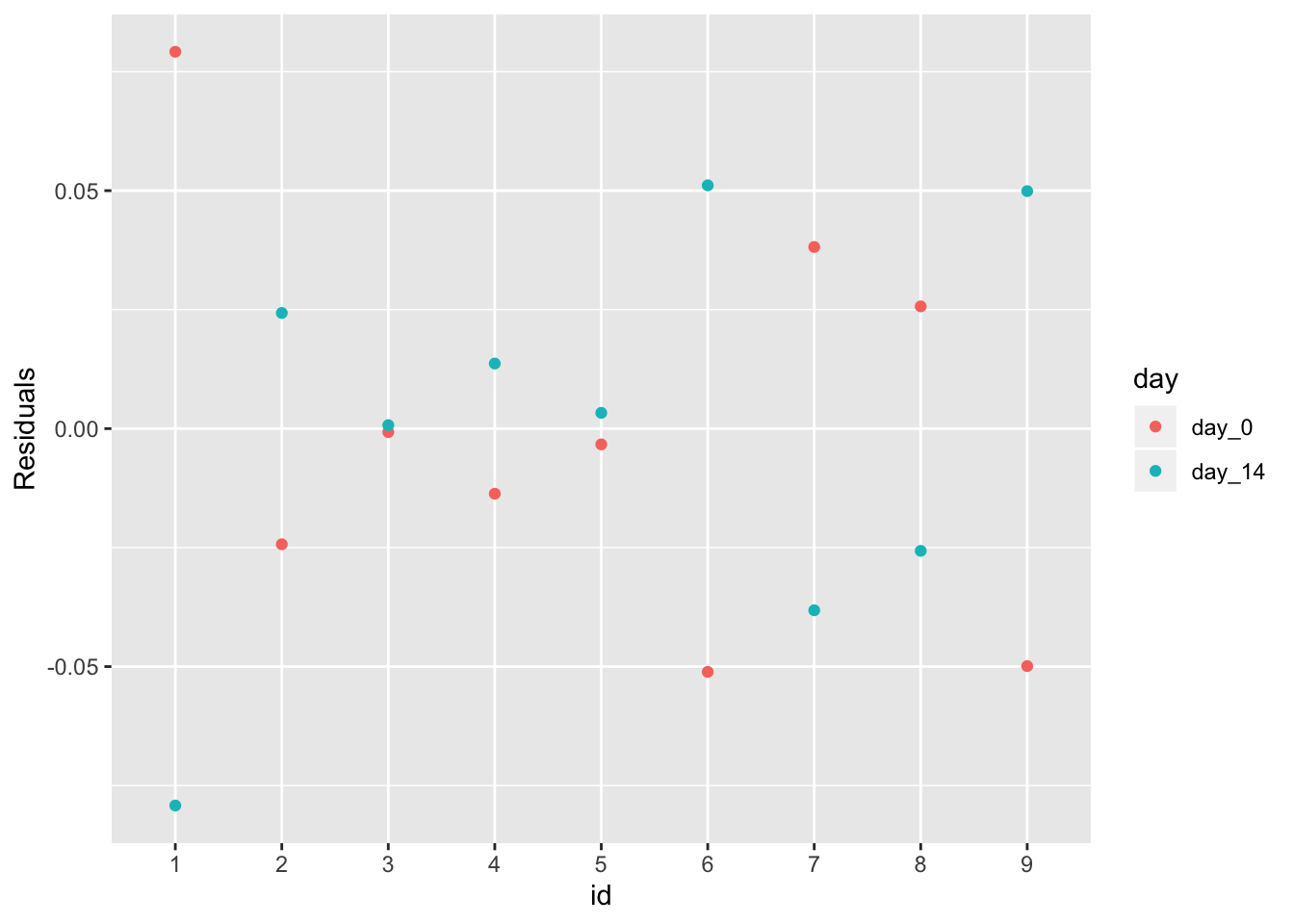
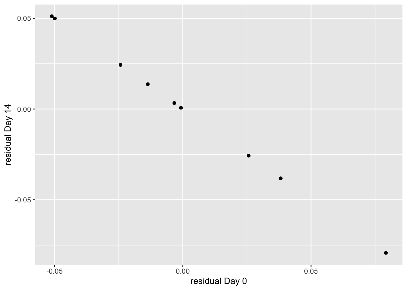
The perfect, negative correlation of the residuals is more explicitly shown with a scatterplot of day_14 residuals vs. day_0 residuals.
conclusion
There is some discussion on twitter and pubpeer on the mechanism of the inflated type I error; is it 1) the unpaired t-test, 2) the transformation, or 3) combination of both? The unpaired t-test is not the mechanism, because without the transformation, the unpaired t-test is conservative (fewer type I error than nominal) not liberal. It is the transformation that inflates the error. But, because of what a paired t-test does (it tests b-a = 0), it is unaffected by the transformation.
