
What is the consequence of a Shapiro-Wilk test-of-normality filter on Type I error and Power?
This 1990-wants-you-back doodle explores the effects of a Normality Filter – using a Shapiro-Wilk (SW) test as a decision rule for using either a t-test or some alternative such as a 1) non-parametric Mann-Whitney-Wilcoxon (MWW) test, or 2) a t-test on the log-transformed response. In this strategy, the alternative is used if the Shapiro-Wilk p-value is less than some cut-off (such as 0.05), otherwise the t-test on the untransformed data is used.
TL;DR – Meh. Using a Shapiro-Wilk filter isn’t going to lead to either better or worse inference. That said, if one simply wants a p-value, there are more powerful methods than a t-test on log-transformed data or Mann-Whitney-Wilcoxan..
And of course, none of this addresses estimation itself, just the NHST approach to discovery. This quote from Lumley et al is relevant:
“The major limitation on the t-test and linear regression for inference about associations is not a distributional one, but whether detecting and estimating a difference in the mean of the outcome answers the scientific question at hand.”1
Motivation teaching applied biostatistics to experimental biologists, who learn to do the shapiro-wilks filter from either a previous course, or more likely, its what they commonly read in the literature
Other literature Lumley et al is relevant and Rochon et al
Stuff that needs to be repeatedly stated The failure to reject a null hypothesis does not mean the null hypothesis is true. Or, in the context of this post, we shouldn’t conclude that a sample is “normal” because a Shapiro-Wilk p-value > 0.05. The logic of a test of normality (or homogeneity) before a t-test/ANOVA, then, isn’t consistent with frequentist thinking. But, maybe we should only think of the Normality filter as an objective model check, compared to, say, inspecting a Q-Q plot.
More stuff that needs to be repeatedly stated It is not uncommon to hear and even read that t-tests assume that the response variable is normally distributed. This is not correct. It is the response conditional on the group that is assumed to be normal. Or, equivalently, it is the residuals from a linear model fit to the data that are assumed to be normal. “Conditional on the group” suggests to some textbook authors that normality should be tested on the response variable in each group seperately. The data pass the Normality filter only if the p-value of the SW test is > 0.05 on both tests. This way of thinking about testing the normal assumption is constraining because it doesn’t allow for adjusting for covariates. A better way to think about testing normality is a single test of the residuals of the fit linear model. This way of thinking is better because it naturally leads to model checking of more complex models.
The Normality filter itself raises a few questions that interest me. Given that the p-value of a t-test is not conditional on “passing” the Normality filter…
What is the probability of rejecting the null conditional on only the subset of true nulls that “pass” the Shapiro-Wilk test (that is, how does the filter change the size or Type I error of the t-test)?
What is the probability of rejecting the null conditional on only the subset of false nulls that pass the Shapiro-Wilk test (that is, how does the filter change the power of the t-test)?
Rochon et al. 2 address #1 with a simulation with data generated using normal, uniform, and exponentitial distributions. I don’t know how relevant the uniform and exponential distributions are for most biological data but the exponential at least has some features in common other skewed distributions with a variance that is a function of the mean, including lognormal and gamma (for continuous responses), and a negative binomial (for count data). Rochon’s implementation used R’s “default” exponential settings but the distribution of the performance statistics (type I error and power) will certainly be conditional on the parameterization of the exponential (or gamma or neg binomial) – that is, how much the data are “approximately” normal.
Set up
library(data.table)
library(MASS)
library(ggplot2)
library(ggpubr)
library(cowplot)

do_sims <- FALSE # redo simulations?
fake_data <- function(niter=10^4, n=50, location=0, scale=1, shape=1, effect=0, dist="normal"){
if(dist=="normal"){
cn <- matrix(rnorm(n*niter, mean=location, sd=scale), nrow=n, ncol=niter)
tr <- matrix(rnorm(n*niter, mean=(location + effect), sd=scale), nrow=n, ncol=niter)
fd <- rbind(cn, tr)
}
if(dist=="nb"){ # negative binomial for counts
cn <- matrix(rnegbin(niter*n, mu=location, theta=shape), nrow=n, ncol=niter)
tr <- matrix(rnegbin(niter*n, mu=(location + effect), theta=shape), nrow=n, ncol=niter)
fd <- rbind(cn, tr)
}
if(dist=="exp"){ # exponential to reproduce paper
rate_cn <- 1/location
rate_tr <- 1/(location + effect)
cn <- matrix(rexp(niter*n, rate=rate_cn), nrow=n, ncol=niter)
tr <- matrix(rexp(niter*n, rate=rate_tr), nrow=n, ncol=niter)
fd <- rbind(cn, tr)
}
if(dist=="lnorm"){ # exponential to reproduce paper
cn <- matrix(rlnorm(niter*n, meanlog=location, sdlog=scale), nrow=n, ncol=niter)
tr <- matrix(rlnorm(niter*n, meanlog=location, sdlog=scale), nrow=n, ncol=niter)
fd <- rbind(cn, tr)
}
return(fd)
}
filter_stats <- function(fd){
# outputs SW p for residual, group1, and group2 + unconditional t-test p
niter <- ncol(fd)
n <- nrow(fd)/2
x <- rep(c("a","b"), each=n)
test_stats_cols <- c("residual", "group1","group2", "p", "p.log", "p.mww")
test_stats <- matrix(NA, nrow=niter, ncol=length(test_stats_cols))
colnames(test_stats) <- test_stats_cols
if(min(fd)==0){
logfd <- log(fd+1)
} else{
logfd <- log(fd) # exponential, gamma
}
iter <- 1 # for debugging
for(iter in 1:niter){
test_stats[iter, "residual"] <- shapiro.test(residuals(lm(fd[, iter] ~ x)))$p.value # using residual
# test_stats[iter, "group1"] <- shapiro.test(fd[1:n, iter])$p.value # using group variable
# test_stats[iter, "group2"] <- shapiro.test(fd[(n+1):(2*n), iter])$p.value # using group variable
test_stats[iter, "p"] <- t.test(fd[, iter] ~ x, var.equal=TRUE)$p.value
test_stats[iter, "p.log"] <- t.test(logfd[, iter] ~ x, var.equal=TRUE)$p.value
test_stats[iter, "p.mww"] <- wilcox.test(fd[, iter] ~ x, exact=FALSE)$p.value
}
return(test_stats)
}
filter_summary <- function(test_stats, alpha=0.05){
# note that prob of at least 1 group rejected is
# 1 - (1-alpha)^2
niter <- nrow(test_stats)
###### Shapiro Wilk test stats
# rate of SW rejection using residual
SW_rej_residual <- sum(test_stats$residual < alpha)/niter
# rate of SW rejection testing each group seperately
#SW_rej_group <- sum(test_stats$group1 < alpha | test_stats$group2 < alpha)/niter # SW positives using group
##### t-test stats
# unconditional type I error/power using t-test
t_unconditional <- sum(test_stats$p < 0.05)/niter
# conditional type I/power of subset that "pass" (not rejected) shapiro wilk test using residuals
t_pass_residual <- sum(test_stats[residual > alpha, p] < 0.05)/sum(test_stats[,residual > alpha])
# conditional type I/power of subset that "pass" (not rejected) shapiro wilk test using groupwise
#t_pass_group <- sum(test_stats[group1 > alpha & group2 > alpha, p] < 0.05)/sum(test_stats[, group1 > alpha & group2 > alpha])
# conditional type I/power of subset that "fail" (rejected) shapiro wilk test using residuals
t_rej_residual <- sum(test_stats[residual < alpha, p] < 0.05)/sum(test_stats[,residual < alpha])
# conditional type I/power of subset that "fail" (rejected) shapiro wilk test using groupwise
#t_rej_group <- sum(test_stats[group1 < alpha | group2 < alpha, p] < 0.05)/sum(test_stats[, group1 < alpha | group2 < alpha]) # conditional on positive SW on group
##### Mann-Whitney-Wilcoxon test stats
# unconditional type I error/power using MWW
mww_unconditional <- sum(test_stats$p.mww < 0.05)/niter
# conditional type I/power of subset that "fail" (rejected) shapiro wilk test using residuals
mww_fail_residual <- sum(test_stats[residual < alpha, p.mww] < 0.05)/sum(test_stats[,residual < alpha])
# conditional type I/power of subset that "fail" (rejected) shapiro wilk test using groupwise
#mww_fail_group <- sum(test_stats[group1 < alpha & group2 < alpha, p.mww] < 0.05)/sum(test_stats[, group1 < alpha & group2 < alpha])
##### combined t-test + Mann-Whitney-Wilcoxon test stats
# conditional type I/power of subset that "pass" (not rejected) shapiro wilk test using residuals
t_mww_fail_residual <- (sum(test_stats[residual > alpha, p] < 0.05) +
sum(test_stats[residual < alpha, p.mww] < 0.05))/niter
# conditional type I/power of subset that "pass" (not rejected) shapiro wilk test using groupwise
#t_mww_fail_group <- (sum(test_stats[group1 > alpha & group2 > alpha, p] < 0.05) +
# sum(test_stats[group1 < alpha & group2 < alpha, p.mww] < 0.05))/niter
##### log-t test stats
logt_unconditional <- sum(test_stats$p.log < 0.05)/niter
# conditional type I/power of subset that "fail" (rejected) shapiro wilk test using residuals
logt_fail_residual <- sum(test_stats[residual < alpha, p.log] < 0.05)/sum(test_stats[,residual < alpha])
# conditional type I/power of subset that "fail" (rejected) shapiro wilk test using groupwise
#logt_fail_group <- sum(test_stats[group1 < alpha & group2 < alpha, p.log] < 0.05)/sum(test_stats[, group1 < alpha & group2 < alpha])
##### combined t-test + log-t test stats
# conditional type I/power of subset that "pass" (not rejected) shapiro wilk test using residuals
t_logt_fail_residual <- (sum(test_stats[residual > alpha, p] < 0.05) +
sum(test_stats[residual < alpha, p.log] < 0.05))/niter
# conditional type I/power of subset that "pass" (not rejected) shapiro wilk test using groupwise
#t_logt_fail_group <- (sum(test_stats[group1 > alpha & group2 > alpha, p] < 0.05) +
# sum(test_stats[group1 < alpha & group2 < alpha, p.log] < 0.05))/niter
res <- c(SW_rej.res=SW_rej_residual,
#SW_rej.group=SW_rej_group,
t.uncond=t_unconditional,
t_pass.res=t_pass_residual,
#t_pass.group=t_pass_group,
t_rej.residual=t_rej_residual,
#t_rej_group=t_rej_group,
mww.uncond=mww_unconditional,
mww_fail.res=mww_fail_residual,
#mww_fail.group=mww_fail_group,
t_mww_fail.res=t_mww_fail_residual,
#t_mww_fail.group=t_mww_fail_group,
logt.uncond=logt_unconditional,
logt_fail.res=logt_fail_residual,
#logt_fail.group=logt_fail_group,
t_logt_fail.res=t_logt_fail_residual
#t_logt_fail.group=t_logt_fail_group
)
return(res)
}Normal distribution
No real data are normally distributed so this parameterization of the simulation gives the behavior of the shapiro-wilk filter for data that are effectively normal.
if(do_sims==TRUE){
  set.seed(1)
  base_niter <- 10^4 # target number of shapiro-wilk tests that "pass" (p > 0.05)

  mu_i <- 10
  sigma_set <- c(1)
  alpha_set <- c(0.1, 0.05, 0.01)
  n_set <- c(10)
  niter_set <- c(base_niter, base_niter*5, base_niter*10) # more iterations to get more samples that "pass" filter
  res_table <- data.table(NULL)
  gg <- list(NULL)
  list_i <- 0
  for(effect_i in c(0, 0.8)){ # "large" effect
    for(sigma_i in sigma_set){
      list_i <- list_i + 1
      for(i in 1:length(n_set)){
        n_i <- n_set[i]
        niter_i <- niter_set[i]
        fd <- fake_data(niter=niter_i, n=n_i, location=mu_i, scale=sigma_i, effect=effect_i, dist="normal")

        res <- data.table(filter_stats(fd))
        for(alpha_i in alpha_set){
          res_table <- rbind(res_table, data.table(
            iter = niter_i,
            mu = mu_i,
            sigma = sigma_i,
            effect = effect_i,
            cn_mean = mean(fd[1:n_i,]),
            cn_sd = sd(fd[1:n_i,]),
            cn_cv = sd(fd[1:n_i,])/mean(fd[1:n_i,]),
            tr_mean = mean(fd[(n_i+1):(n_i*2),]),
            tr_sd = sd(fd[(n_i+1):(n_i*2),]),
            tr_cv = sd(fd[(n_i+1):(n_i*2),])/mean(fd[(n_i+1):(n_i*2),]),
            n = n_i,
            alpha = alpha_i,
            data.table(t(filter_summary(res, alpha=alpha_i)))))
        }
      }
    }
  }
  norm_table <- t(res_table)
  # write to file
  write.table(norm_table, "../output/2019-08-08-norm_table.txt",quote=FALSE, sep="\t")
}else{ # if not true, read file
  norm_table <- read.table("../output/2019-08-08-norm_table.txt", header=TRUE, sep="\t")
}
Type I error
type1 <- norm_table[, 1:3]
colnames(type1) <- c("n=6", "n=10", "n=20")
row.names(type1) <- c(
  "iterations",
  "mu",
  "sigma",
  "effect",
  "Cn mean",
  "Cn sd",
  "Cn cv",
  "Tr mean",
  "Tr sd",
  "Tr cv",
  "n",
  "alpha for normality test",
  "failed normality, rate",
  "t-test: type I, unconditional",
  "t-test: type I, | pass",
  "t-test: type I, | fail",
  "MWW-test: type I, unconditional",
  "MWW-test: type I, | fail",
  "t-MWW: type I",
  "log t-test: type I, unconditional",
  "log t-test: type I, | fail",
  "t-log t: type I"
)
knitr::kable(type1, digits=3, caption="Type I error as a function of n for normal data")| n=6 | n=10 | n=20 | |
|---|---|---|---|
| iterations | 10000.000 | 10000.000 | 10000.000 |
| mu | 10.000 | 10.000 | 10.000 |
| sigma | 1.000 | 1.000 | 1.000 |
| effect | 0.000 | 0.000 | 0.000 |
| Cn mean | 9.998 | 9.998 | 9.998 |
| Cn sd | 1.004 | 1.004 | 1.004 |
| Cn cv | 0.100 | 0.100 | 0.100 |
| Tr mean | 10.001 | 10.001 | 10.001 |
| Tr sd | 1.001 | 1.001 | 1.001 |
| Tr cv | 0.100 | 0.100 | 0.100 |
| n | 10.000 | 10.000 | 10.000 |
| alpha for normality test | 0.100 | 0.050 | 0.010 |
| failed normality, rate | 0.097 | 0.047 | 0.010 |
| t-test: type I, unconditional | 0.048 | 0.048 | 0.048 |
| t-test: type I, | pass | 0.048 | 0.049 | 0.048 |
| t-test: type I, | fail | 0.044 | 0.036 | 0.021 |
| MWW-test: type I, unconditional | 0.040 | 0.040 | 0.040 |
| MWW-test: type I, | fail | 0.058 | 0.055 | 0.073 |
| t-MWW: type I | 0.049 | 0.049 | 0.048 |
| log t-test: type I, unconditional | 0.048 | 0.048 | 0.048 |
| log t-test: type I, | fail | 0.045 | 0.038 | 0.042 |
| t-log t: type I | 0.048 | 0.048 | 0.048 |
Summary:
- The conditional Type I error of the t-test for the sets that pass the Shapiro-Wilk filter is effectively the nominal value (0.05), as is that for the the unconditional Type I. The conditional Type I error for the sets that fail the filter is small (the test is conservative) but this is irrelevant because these data would be analyzed by Mann-Whitney-Wilcoxon or by a t-test of log-transformed data.
- The conditional Type I error for MWW test for sets that fail the Shapiro-Wilk filter is very slightly liberal.
- The overal Type I error for the normality-test filter strategy using the Mann-Whitney-Wilcoxon as the alternative is effectively 0.05
- The results using the t-test of log transform are very close to nominal regardless of strategy.
These results replicate that in Rochon et al. See also Lumley et al (both are cited above)
Power
type2 <- norm_table[, 4:6] # really power, not type 2
colnames(type2) <- c("n=6", "n=10", "n=20")
row.names(type2) <- c(
  "iterations",
  "mu",
  "sigma",
  "effect",
  "Cn mean",
  "Cn sd",
  "Cn cv",
  "Tr mean",
  "Tr sd",
  "Tr cv",
  "n",
  "alpha for normality test",
  "failed normality, rate",
  "t-test: power, unconditional",
  "t-test: power, | pass",
  "t-test: power, | fail",
  "MWW-test: power, unconditional",
  "MWW-test: power, | fail",
  "t-MWW: power",
  "log t-test: power, unconditional",
  "log t-test: power, | fail",
  "t-log t: power"
)
knitr::kable(type2, digits=3, caption="Power as a function of n for normal data")| n=6 | n=10 | n=20 | |
|---|---|---|---|
| iterations | 10000.000 | 10000.000 | 10000.000 |
| mu | 10.000 | 10.000 | 10.000 |
| sigma | 1.000 | 1.000 | 1.000 |
| effect | 0.800 | 0.800 | 0.800 |
| Cn mean | 10.000 | 10.000 | 10.000 |
| Cn sd | 0.997 | 0.997 | 0.997 |
| Cn cv | 0.100 | 0.100 | 0.100 |
| Tr mean | 10.799 | 10.799 | 10.799 |
| Tr sd | 0.999 | 0.999 | 0.999 |
| Tr cv | 0.093 | 0.093 | 0.093 |
| n | 10.000 | 10.000 | 10.000 |
| alpha for normality test | 0.100 | 0.050 | 0.010 |
| failed normality, rate | 0.104 | 0.051 | 0.008 |
| t-test: power, unconditional | 0.394 | 0.394 | 0.394 |
| t-test: power, | pass | 0.396 | 0.395 | 0.394 |
| t-test: power, | fail | 0.376 | 0.377 | 0.412 |
| MWW-test: power, unconditional | 0.354 | 0.354 | 0.354 |
| MWW-test: power, | fail | 0.409 | 0.433 | 0.538 |
| t-MWW: power | 0.398 | 0.397 | 0.395 |
| log t-test: power, unconditional | 0.393 | 0.393 | 0.393 |
| log t-test: power, | fail | 0.377 | 0.383 | 0.388 |
| t-log t: power | 0.394 | 0.394 | 0.394 |
Summary:
- The unconditional Mann-Whitney-Wilcoxon has slightly reduced power relative to the unconditional t-test on either untransformed or log transformed response.
- The Mann-Whitney-Wilcoxon for sets that fail has slightly greater power relative to the unconditional t-test on either untransformed or log transformed response.
- The combination of 1 and 2 mean that the unconditional t-test, the normality-test filter strategy using Mann-Whitney-Wilcoxon as the alternative, the unconditional t-test on log-transformed responses, and the the normality-test filter strategy using log transformed response as the alternative all have effectively equivalent power.
Right skewed continuous – lognormal
The lognormal distribution is explored with two parameterizations, one with larger skew and one with smaller skew, but still distinct from Normal.
if(do_sims==TRUE){
  set.seed(1)
  base_niter <- 10^4 # target number of shapiro-wilk tests that "pass" (p > 0.05)
  mean_cn <- 10
  sd_cn <- 2
  effect_i <- 2

  mu_i <- 0 # exp(x) = 1
  sigma_set <- c(0.8, 0.4)
  alpha_set <- c(0.05)
  n_set <- c(6, 10, 20)
  niter_set <- c(base_niter, base_niter*5, base_niter*10) # more iterations to get more samples that "pass" filter
  res_table <- data.table(NULL)
  gg <- list(NULL)
  list_i <- 0
  for(effect_i in c(0, sd_cn*0.8)){ # "large" effect
    for(sigma_i in sigma_set){
      for(n_i in 1:length(n_set)){
        list_i <- list_i + 1
        niter_i <- niter_set[i]
        fd <- fake_data(niter=niter_i, n=n_i, location=mu_i, scale=sigma_i, effect=0, dist="lnorm")

        # set to common CV
        # sd = CV x Mean
        fd <- scale(fd, scale=TRUE)
        sd_cn <- 2
        fd[1:n_i,] <- fd[1:n_i,]*sd_cn + mean_cn # 2 is the sd in the CN
        fd[(n_i+1):(n_i*2),] <- fd[(n_i+1):(n_i*2),]*sd_cn*(mean_cn + effect_i)/mean_cn + mean_cn + effect_i

        if(n_i == n_set[length(n_set)] & effect_i==0){
          gg_fd <- data.table(x=rep(c("a","b"), each=n_i), fd[, 1:3])
          gg0 <- gghistogram(c(fd))
          gg1 <- ggboxplot(data=gg_fd, x="x", y="V1", add="jitter")
          gg2 <- ggboxplot(data=gg_fd, x="x", y="V2", add="jitter")
          gg3 <- ggboxplot(data=gg_fd, x="x", y="V3", add="jitter")
          gg <- plot_grid(gg0, gg1, gg2, gg3, ncol=4, rel_widths = c(2, 1, 1, 1, 1))
          plot_file_name <- paste0("../images/2019-08-08-gg-s=", sigma_i, ".png")
          save_plot(plot_file_name, gg, base_height = 4, base_width=6)
        }

        res <- data.table(filter_stats(fd))
        for(alpha_i in alpha_set){
          res_table <- rbind(res_table, data.table(
            iter = niter_i,
            mu = mu_i,
            sigma = sigma_i,
            effect = effect_i,
            cn_mean = mean(fd[1:n_i,]),
            cn_sd = sd(fd[1:n_i,]),
            cn_cv = sd(fd[1:n_i,])/mean(fd[1:n_i,]),
            tr_mean = mean(fd[(n_i+1):(n_i*2),]),
            tr_sd = sd(fd[(n_i+1):(n_i*2),]),
            tr_cv = sd(fd[(n_i+1):(n_i*2),])/mean(fd[(n_i+1):(n_i*2),]),
            n = n_i,
            alpha = alpha_i,
            #  alpha_2 = 1-(1-alpha_i)^2,
            data.table(t(filter_summary(res, alpha=alpha_i)))))
        }
      }
    }
  }
  lognorm_table <- t(res_table)
  # write to file
  write.table(lognorm_table, "../output/2019-08-08-lognorm_table.txt",quote=FALSE, sep="\t")
}else{ # if not true, read file
  lognorm_table <- read.table("../output/2019-08-08-lognorm_table.txt", header=TRUE, sep="\t")
}
What the parameterizations look like
knitr::include_graphics("2019-08-08-what-is-the-consequence-of-a-shapiro-wilk-test-of-normality-filter-on-type-i-error-and-power_files/figure-html/2019-08-08-gg-s=0.8.png")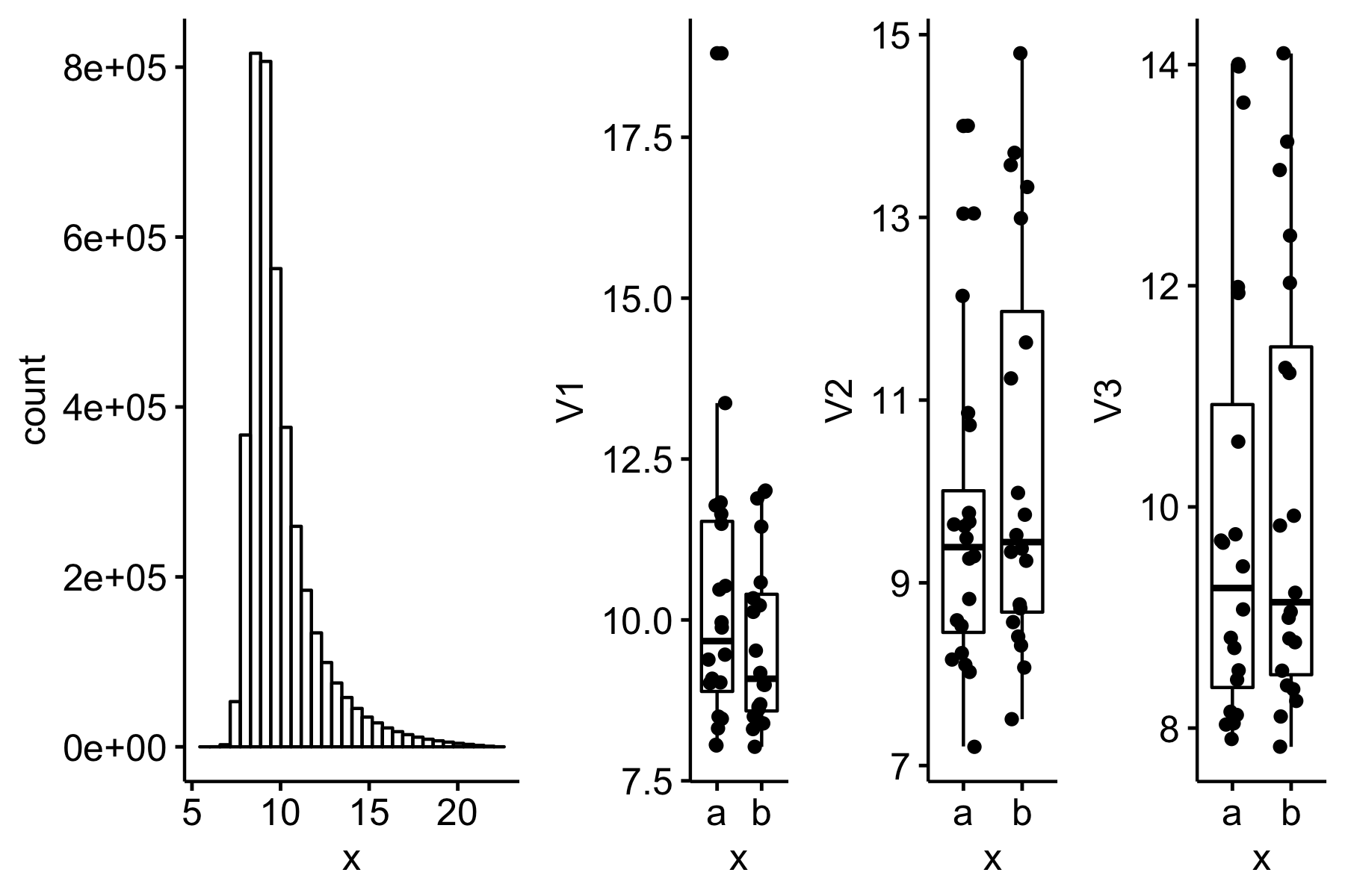
Figure 1: sigma = 0.8 (less approximately normal)
knitr::include_graphics("2019-08-08-what-is-the-consequence-of-a-shapiro-wilk-test-of-normality-filter-on-type-i-error-and-power_files/figure-html/2019-08-08-gg-s=0.4.png")
Figure 2: sigma = 0.4 (more approximately normal)
Type I error
type1 <- lognorm_table[, 1:6]
colnames(type1) <- c("n=6, sigma=.8", "n=10, sigma=.8", "n=20, sigma=.8", "n=6, sigma=.4", "n=10, sigma=.4", "n=20, sigma=.4")
row.names(type1) <- c(
  "iterations",
  "mu",
  "sigma",
  "effect",
  "Cn mean",
  "Cn sd",
  "Cn cv",
  "Tr mean",
  "Tr sd",
  "Tr cv",
  "n",
  "alpha for normality test",
  "failed normality, rate",
  "t-test: type I, unconditional",
  "t-test: type I, | pass",
  "t-test: type I, | fail",
  "MWW-test: type I, unconditional",
  "MWW-test: type I, | fail",
  "t-MWW: type I",
  "log t-test: type I, unconditional",
  "log t-test: type I, | fail",
  "t-log t: type I"
)
knitr::kable(type1, digits=3, caption="Type I error as a function of n and sigma for lognormal data")| n=6, sigma=.8 | n=10, sigma=.8 | n=20, sigma=.8 | n=6, sigma=.4 | n=10, sigma=.4 | n=20, sigma=.4 | |
|---|---|---|---|---|---|---|
| iterations | 10000.000 | 50000.000 | 100000.000 | 10000.000 | 50000.000 | 100000.000 |
| mu | 0.000 | 0.000 | 0.000 | 0.000 | 0.000 | 0.000 |
| sigma | 0.800 | 0.800 | 0.800 | 0.400 | 0.400 | 0.400 |
| effect | 0.000 | 0.000 | 0.000 | 0.000 | 0.000 | 0.000 |
| Cn mean | 9.992 | 9.995 | 10.001 | 9.998 | 9.994 | 10.001 |
| Cn sd | 1.912 | 1.948 | 1.976 | 1.912 | 1.949 | 1.976 |
| Cn cv | 0.191 | 0.195 | 0.198 | 0.191 | 0.195 | 0.198 |
| Tr mean | 10.008 | 10.005 | 9.999 | 10.002 | 10.006 | 9.999 |
| Tr sd | 1.917 | 1.951 | 1.973 | 1.918 | 1.950 | 1.974 |
| Tr cv | 0.192 | 0.195 | 0.197 | 0.192 | 0.195 | 0.197 |
| n | 6.000 | 10.000 | 20.000 | 6.000 | 10.000 | 20.000 |
| alpha for normality test | 0.050 | 0.050 | 0.050 | 0.050 | 0.050 | 0.050 |
| failed normality, rate | 0.413 | 0.742 | 0.982 | 0.155 | 0.318 | 0.653 |
| t-test: type I, unconditional | 0.035 | 0.038 | 0.044 | 0.045 | 0.046 | 0.049 |
| t-test: type I, | pass | 0.054 | 0.093 | 0.230 | 0.049 | 0.057 | 0.072 |
| t-test: type I, | fail | 0.008 | 0.019 | 0.040 | 0.022 | 0.025 | 0.036 |
| MWW-test: type I, unconditional | 0.040 | 0.042 | 0.049 | 0.041 | 0.042 | 0.049 |
| MWW-test: type I, | fail | 0.029 | 0.035 | 0.047 | 0.042 | 0.041 | 0.044 |
| t-MWW: type I | 0.044 | 0.050 | 0.050 | 0.048 | 0.052 | 0.054 |
| log t-test: type I, unconditional | 0.039 | 0.043 | 0.047 | 0.048 | 0.048 | 0.049 |
| log t-test: type I, | fail | 0.014 | 0.025 | 0.044 | 0.030 | 0.032 | 0.040 |
| t-log t: type I | 0.038 | 0.043 | 0.048 | 0.046 | 0.049 | 0.051 |
Summary:
- All unconditional tests are slightly conservative (the Mann-Whitney-Wilcoxon least so)
- The conditional Type I error of the t-test for the sets that pass the Shapiro-Wilk filter increases with \(n\) but the rate of this increase is less for the parameterization generating data that is more approximately normal (mu = 0, sigma = 0.4)
- The overal Type I error for the normality-test filter strategy using the Mann-Whitney-Wilcoxon as the alternative is effectively the nominal value (0.05), or maybe a bit conservative at small \(n\) (0.044), regardless of the lognormal parameterization (over the small set explored)
- The overal Type I error for the normality-test filter strategy using the log transformed response as the alternative is effectively the nominal value (0.05), or maybe a bit conservative at small \(n\) (0.038), regardless of the lognormal parameterization (over the small set explored)
Power
type2 <- lognorm_table[, 7:12] # really power, not type 2
colnames(type2) <- c("n=6, sigma=.8", "n=10, sigma=.8", "n=20, sigma=.8", "n=6, sigma=.4", "n=10, sigma=.4", "n=20, sigma=.4")
row.names(type2) <- c(
  "iterations",
  "mu",
  "sigma",
  "effect",
  "Cn mean",
  "Cn sd",
  "Cn cv",
  "Tr mean",
  "Tr sd",
  "Tr cv",
  "n",
  "alpha for normality test",
  "failed normality, rate",
  "t-test: power, unconditional",
  "t-test: power, | pass",
  "t-test: power, | fail",
  "MWW-test: power, unconditional",
  "MWW-test: power, | fail",
  "t-MWW: power",
  "log t-test: power, unconditional",
  "log t-test: power, | fail",
  "t-log t: power"
)
knitr::kable(type2, digits=3, caption="Power as a function of n and sigma for lognormal response")| n=6, sigma=.8 | n=10, sigma=.8 | n=20, sigma=.8 | n=6, sigma=.4 | n=10, sigma=.4 | n=20, sigma=.4 | |
|---|---|---|---|---|---|---|
| iterations | 10000.000 | 50000.000 | 100000.000 | 10000.000 | 50000.000 | 100000.000 |
| mu | 0.000 | 0.000 | 0.000 | 0.000 | 0.000 | 0.000 |
| sigma | 0.800 | 0.800 | 0.800 | 0.400 | 0.400 | 0.400 |
| effect | 1.600 | 1.600 | 1.600 | 1.600 | 1.600 | 1.600 |
| Cn mean | 9.997 | 9.995 | 10.001 | 9.998 | 9.994 | 10.001 |
| Cn sd | 1.913 | 1.948 | 1.976 | 1.912 | 1.949 | 1.976 |
| Cn cv | 0.191 | 0.195 | 0.198 | 0.191 | 0.195 | 0.198 |
| Tr mean | 11.603 | 11.605 | 11.599 | 11.602 | 11.606 | 11.599 |
| Tr sd | 2.224 | 2.263 | 2.289 | 2.224 | 2.262 | 2.290 |
| Tr cv | 0.192 | 0.195 | 0.197 | 0.192 | 0.195 | 0.197 |
| n | 6.000 | 10.000 | 20.000 | 6.000 | 10.000 | 20.000 |
| alpha for normality test | 0.050 | 0.050 | 0.050 | 0.050 | 0.050 | 0.050 |
| failed normality, rate | 0.398 | 0.739 | 0.980 | 0.157 | 0.317 | 0.647 |
| t-test: power, unconditional | 0.180 | 0.326 | 0.610 | 0.180 | 0.321 | 0.612 |
| t-test: power, | pass | 0.219 | 0.400 | 0.689 | 0.189 | 0.333 | 0.614 |
| t-test: power, | fail | 0.121 | 0.301 | 0.608 | 0.137 | 0.295 | 0.611 |
| MWW-test: power, unconditional | 0.245 | 0.491 | 0.849 | 0.175 | 0.332 | 0.661 |
| MWW-test: power, | fail | 0.288 | 0.533 | 0.852 | 0.225 | 0.415 | 0.703 |
| t-MWW: power | 0.246 | 0.498 | 0.849 | 0.194 | 0.359 | 0.672 |
| log t-test: power, unconditional | 0.225 | 0.392 | 0.728 | 0.199 | 0.350 | 0.660 |
| log t-test: power, | fail | 0.202 | 0.384 | 0.728 | 0.196 | 0.365 | 0.678 |
| t-log t: power | 0.212 | 0.388 | 0.728 | 0.190 | 0.343 | 0.656 |
Summary:
- The unconditional t-test of log transfored response and especially Mann-Whitney-Wilcoxon have more power than the unconditional t-test.
- The overal power of the normality-test filter strategy using the Mann-Whitney-Wilcoxon as the alternative is about the same as the unconditional MWW strategy with the more skewed parameterization but slightly higher than that for the unconditional MWW strategy with the less skewed parameterization.
- The overal power of the normality-test filter strategy using the log transformation as the alternative is about the same as the unconditional log transformation strategy regardless of the parameterization of the lognormal (over the space of my parameterization)
Lumley, T., Diehr, P., Emerson, S., & Chen, L. (2002). The Importance of the Normality Assumption in Large Public Health Data Sets. Annual Review of Public Health, 23(1), 151–169. https://doi.org/10.1146/annurev.publhealth.23.100901.140546↩
Rochon, J., Gondan, M., & Kieser, M. (2012). To test or not to test: Preliminary assessment of normality when comparing two independent samples. BMC Medical Research Methodology, 12(1). https://doi.org/10.1186/1471-2288-12-81↩
