Update to the earlier post, which was written in response to my own thinking about how to teach stastics to experimental biologists working in fields that are dominated by hypothesis testing instead of estimation. That is, should these researchers learn GLMs or is a t-test on raw or log-transformed data on something like count data good enough – or even superior? My post was written without the benefit of either [Ives](Ives, Anthony R. “For testing the significance of regression coefficients, go ahead and log‐transform count data.” Methods in Ecology and Evolution 6, no. 7 (2015): 828-835) or Warton et al.. With hindsight, I do vaguely recall Ives, and my previous results support his conclusions, but I was unaware of Warton.

Warton et al is a fabulous paper. A must read. A question that I have is, under the null isn’t the response itself exchangeable, so that residuals are unnecessary? Regardless, the implementation in the mvabund package is way faster than my own R-scripted permutation. So here is my earlier simulation in light of Warton et al.

TL;DR – If we live and die by NHST, then we want to choose a test with good Type I error control but has high power. The quasi-poisson both estimates an interpretable effect (unlike a t-test of log(y +1)) and has good Type I control with high power.

A bit longer: The quasi-poisson LRT and the permutation NB have good Type I control and high power. The NB Wald and LRT have too liberal Type I control. The t-test of log response has good Type I control and high power at low \(n\) but is slightly inferior to the glm with increased \(n\). The t-test, Welch, and Wilcoxan have conservative Type I control. Of these, the Wilcoxan has higher power than the t-test and Welch but not as high as the GLMs or log-transformed response.

load libraries

library(ggplot2)
library(ggpubr)
library(MASS)
library(mvabund)
library(lmtest)
library(nlme)
library(data.table)
library(cowplot)

The simulation

Single factor with two levels and a count (negative binomial) response.
theta (shape parameter of NB) = 0.5
Relative effect sizes of 0%, 100%, and 200%
Ref count of 4
\(n\) of 5 and 10

p-values computed from

t-test on raw response
Welch t-test on raw response
t-test on log transformed response
Wilcoxan test
glm with negative binomial family and log-link using Wald test
glm with negative binomial family and log-link using LRT
glm with negative binomial family and permutation test (using PIT residuals)¹
glm with quasi-poisson family and log-link using LRT

do_sim <- function(sim_space=NULL, niter=1000, nperm=1000, algebra=FALSE){
  # the function was run with n=1000 and the data saved. on subsequent runs
  # the data are loaded from a file
  # the function creates three different objects to return, the object
  # return is specified by "return_object" = NULL, plot_data1, plot_data2
  
  set.seed(1)
  
  methods <- c("t", "Welch", "log", "Wilcoxan", "nb", "nb.x2", "nb.perm", "qp")
  p_table <- data.table(NULL)
  
  if(is.null(sim_space)){
    mu_0_list <- c(4) # control count
    theta_list <- c(0.5) # dispersion
    effect_list <- c(1) # effect size will be 1X, 1.5X, 2X, 3X
    n_list <- c(10) # sample size
    sim_space <- data.table(expand.grid(theta=theta_list, mu_0=mu_0_list, effect=effect_list, n=n_list))
  }
  
  res_table <- data.table(NULL)
  i <- 1 # this is just for debugging
  for(i in 1:nrow(sim_space)){
    # construct clean results table 
    p_table_part <- matrix(NA, nrow=niter, ncol=length(methods))
    colnames(p_table_part) <- methods
    
    # parameters of simulation
    theta_i <- sim_space[i, theta]
    mu_0_i <- sim_space[i, mu_0]
    effect_i <- sim_space[i, effect]
    n_i <- sim_space[i, n]
    treatment <- rep(c("Cn", "Trt"), each=n_i)
    fd <- data.table(treatment=treatment)
    
    # mu (using algebra)
    if(algebra==TRUE){
      X <- model.matrix(~treatment)
      beta_0 <- log(mu_0_i)
      beta_1 <- log(effect_i*mu_0_i) - beta_0
      beta <- c(beta_0, beta_1)
      mu_i <- exp((X%*%beta)[,1])
    }else{ #  using R
      mu_vec <- c(mu_0_i, mu_0_i*effect_i)
      mu_i <- rep(mu_vec, each=n_i)
    }
    nb.error <- numeric(niter)
    
    for(iter in 1:niter){
      set.seed(niter*(i-1) + iter)
      fd[, y:=rnegbin(n=n_i*2, mu=mu_i, theta=theta_i)]
      fd[, log_yp1:=log10(y+1)]
      
      p.t <- t.test(y~treatment, data=fd, var.equal=TRUE)$p.value
      p.welch <- t.test(y~treatment, data=fd, var.equal=FALSE)$p.value
      p.log <- t.test(log_yp1~treatment, data=fd, var.equal=TRUE)$p.value
      p.wilcox <- wilcox.test(y~treatment, data=fd, exact=FALSE)$p.value
      
      # weighted lm, this will be ~same as welch for k=2 groups
      # fit <- gls(y~treatment, data=fd, weights = varIdent(form=~1|treatment), method="ML")
      # p.wls <- coef(summary(fit))["treatmentTrt", "p-value"]
      
      # negative binomial
      # default test using summary is Wald.
      # anova(fit) uses chisq of sequential fit, but using same estimate of theta
      # anova(fit2, fit1), uses chisq but with different estimate of theta
      # lrtest(fit) same as anova(fit2, fit1)
      
      # m1 <- glm.nb(y~treatment, data=fd)
      # m0 <- glm.nb(y~1, data=fd)
      # p.nb.x2 <- anova(m0, m1)[2, "Pr(Chi)"]
      # lr <- 2*(logLik(m1) - logLik(m0))
      # df.x2 = m0$df.residual-m1$df.residual
      # p.nb.x2 <- pchisq(lr, df=df.x2, lower.tail = F)
                
      m1 <- manyglm(y~treatment, data=fd) # default theta estimation "PHI"
      m0 <- manyglm(y~1, data=fd)
      lr <- 2*(logLik(m1) - logLik(m0))
      df.x2 = m0$df.residual-m1$df.residual
      p.nb <- coef(summary(m1))["treatmentTrt", "Pr(>wald)"] # Wald
      p.nb.x2 <- as.numeric(pchisq(lr, df=df.x2, lower.tail = F))
      p.nb.perm <- (anova(m0, m1, nBoot=nperm, show.time='none', p.uni="unadjusted")$uni.p)[2,1]

      # p.nb.x2 <- lrtest(fit)[2, "Pr(>Chisq)"] # doesn't work with a data.table
      
      # quasipoisson
      fit <- glm(y~treatment, data=fd, family=quasipoisson)
      p.qp <- coeftest(fit)[2, "Pr(>|z|)"]
      
      p_table_part[iter,] <- c(p.t, p.welch, p.log, p.wilcox, p.nb, p.nb.x2, p.nb.perm, p.qp)
      
    } # niter
    p_table <- rbind(p_table, data.table(combo=i,
                                         mu_0=mu_0_i,
                                         effect=effect_i,
                                         n=n_i,
                                         theta=theta_i,
                                         nb.error=nb.error,
                                         p_table_part))
    
  } # combos
  
  return(p_table)
}

# Algebra is slower (duh!)
# start_time <- Sys.time()
# do_sim(niter=niter, algebra=FALSE)
# end_time <- Sys.time()
# end_time - start_time
# 
# start_time <- Sys.time()
# do_sim(niter=niter, algebra=TRUE)
# end_time <- Sys.time()
# end_time - start_time

n_iter <- 2000
n_perm <- 2000
mu_0_list <- c(4) # control count
theta_list <- c(0.5) # dispersion
effect_list <- c(1, 2, 4) # effect size will be 1X, 1.5X, 2X, 3X
n_list <- c(5, 10) # sample size
sim_space <- data.table(expand.grid(theta=theta_list, mu_0=mu_0_list, effect=effect_list, n=n_list))

do_it <- FALSE # if FALSE the results are available as a file
if(do_it==TRUE){
  p_table <- do_sim(sim_space, niter=n_iter, nperm=n_perm)
  write.table(p_table, "../output/glm-v-lm.0004.txt", row.names = FALSE, quote=FALSE)
}else{
  p_table <- fread("../output/glm-v-lm.0001.txt")
  p_table[, combo:=paste(effect, n, sep="-")]
  ycols <- setdiff(colnames(p_table), c("combo", "mu_0", "effect", "n", "theta"))
  res_table <- data.table(NULL)
  for(i in p_table[, unique(combo)]){
    p_table_part <- p_table[combo==i, ]
    mu_0_i <- p_table_part[1, mu_0]
    effect_i <- p_table_part[1, effect]
    n_i <- p_table_part[1, n]
    theta_i <- p_table_part[1, theta]
    n_iter_i <- nrow(p_table_part)
    p_sum <- apply(p_table_part[, .SD, .SDcols=ycols], 2, function(x) length(which(x <= 0.05))/n_iter_i)
    res_table <- rbind(res_table, data.table(mu_0 = mu_0_i,
                                             effect = effect_i,
                                             n = n_i,
                                             theta = theta_i,
                                             t(p_sum)))    
  }
  res_table[, n:=factor(n)]
}

Type I error

Key: 1. “nb” uses the Wald test of negative binomial model. 2. “nb.x2” uses the LRT of negative binomial model. 3. “nb.perm” uses a permutation test on PIT residuals of negative binomial model 4. qp uses a LRT of quasi-poisson model

knitr::kable(res_table[effect==1,],
             caption = "Type 1 error as a function of n")

Table 1: Type 1 error as a function of n
mu_0	effect	n	theta	nb.error	t	Welch	log	Wilcoxan	nb	nb.x2	nb.perm	qp
4	1	5	0.5	1	0.032	0.0175	0.0475	0.0270	0.1280	0.1015	0.0515	0.054
4	1	10	0.5	1	0.036	0.0295	0.0505	0.0435	0.0675	0.0695	0.0460	0.053

Power

knitr::kable(res_table[effect!=1,],
             caption = "Power as a function of n")

Table 2: Power as a function of n
mu_0	effect	n	theta	nb.error	t	Welch	log	Wilcoxan	nb	nb.x2	nb.perm	qp
4	2	5	0.5	1	0.0465	0.0240	0.0845	0.0540	0.1710	0.1565	0.0825	0.0960
4	4	5	0.5	1	0.1055	0.0475	0.1950	0.1310	0.3310	0.3295	0.1860	0.1800
4	2	10	0.5	1	0.0900	0.0750	0.1150	0.1025	0.1730	0.1850	0.1285	0.1480
4	4	10	0.5	1	0.3120	0.2600	0.3780	0.3235	0.5255	0.5345	0.4190	0.4405

plots

res <- melt(res_table, 
            id.vars=c("mu_0", "effect", "n", "theta", "nb.error"),
            measure.vars=c("t", "Welch", "log", "Wilcoxan", "nb", "nb.x2", "nb.perm", "qp"),
            variable.name="model",
            value.name="frequency")

gg <- ggplot(data=res[effect==1,], aes(x=n, y=frequency, group=model, color=model)) +
  geom_line() +
  facet_grid(. ~ effect, labeller=label_both) +
  NULL
gg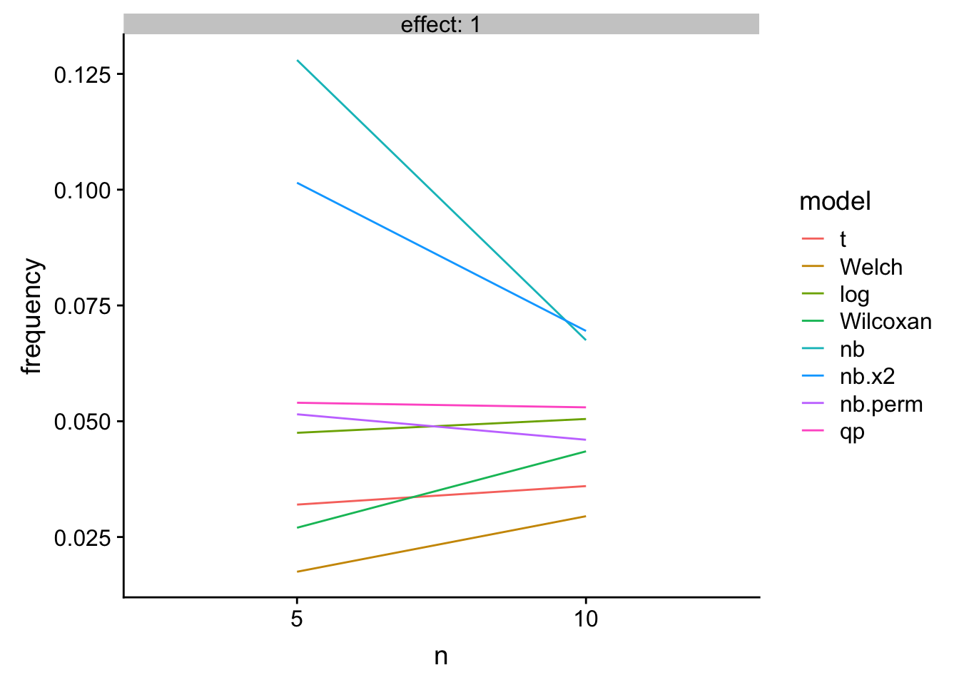

Figure 1: Type I error

gg <- ggplot(data=res[effect!=1,], aes(x=n, y=frequency, group=model, color=model)) +
  geom_line() +
  facet_grid(. ~ effect, labeller=label_both) +
  NULL
gg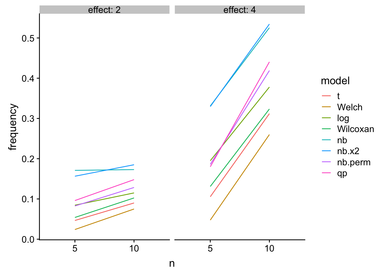

Figure 2: Power

Warton, D.I., Thibaut, L., Wang, Y.A., 2017. The PIT-trap—A “model-free” bootstrap procedure for inference about regression models with discrete, multivariate responses. PLOS ONE 12, e0181790. https://doi.org/10.1371/journal.pone.0181790 ↩

GLM vs. t-tests vs. non-parametric tests if all we care about is NHST -- Update

load libraries

The simulation

Type I error

Power

plots

R doodles. Some ecology. Some physiology. Much fake data.

GLM vs. t-tests vs. non-parametric tests if all we care about is NHST -- Update

load libraries

The simulation

Type I error

Power

plots

R doodles. Some ecology. Some physiology. Much fake data.

How to make plots with factor levels below the x-axis (bench-biology style)

What is an interaction?

How to estimate synergism or antagonism

Type 3 ANOVA in R -- an easy way to publish wrong tables

Linear models with a covariate ("ANCOVA")

Normal Q-Q plots - what is the robust line and should we prefer it?

ANCOVA when the covariate is a mediator affected by treatment

Bootstrap confidence intervals when sample size is really small

What is the consequence of normalizing by each case in the control?

Melting a list of columns