A skeleton simulation of different strategies for NHST for count data if all we care about is a p-value, as in bench biology where p-values are used to simply give one confidence that something didn’t go terribly wrong (similar to doing experiments in triplicate – it’s not the effect size that matters only “we have experimental evidence of a replicable effect”).

tl;dr - At least for Type I error at small \(n\), log(response) and Wilcoxan have the best performance over the simulation space. T-test is a bit conservative. Welch is even more conservative. glm-nb is too liberal.

load libraries

library(ggplot2)
library(ggpubr)
library(MASS)
library(data.table)
library(cowplot)

The simulation

Single factor with two levels and a count (negative binomial) response.
theta (shape parameter) set to 0.5, 1, 100
Relative effect sizes of 0%, 50%, 100%, and 200%
Ref count of 4, 10, 100
\(n\) of 5, 10, 20, 40

p-values computed from

t-test on raw response
Welch t-test on raw response
t-test on log transformed response
Wilcoxan test
glm with negative binomial family and log-link

do_sim <- function(niter=1, return_object=NULL){
  # the function was run with n=1000 and the data saved. on subsequent runs
  # the data are loaded from a file
  # the function creates three different objects to return, the object
  # return is specified by "return_object" = NULL, plot_data1, plot_data2
  methods <- c("t", "Welch", "log", "Wilcoxan", "nb")
  p_table_part <- matrix(NA, nrow=niter, ncol=length(methods))
  colnames(p_table_part) <- methods
  p_table <- data.table(NULL)
  
  res_table <- data.table(NULL)
  beta_0_list <- c(4, 10, 100) # control count
  theta_list <- c(0.5, 1, 100) # dispersion
  effect_list <- c(1:3, 5) # relative effect size will be 0%, 50%, 100%, 200%
  n_list <- c(5, 10, 20, 40) # sample size
  n_rows <- length(beta_0_list)*length(theta_list)*length(effect_list)*length(n_list)*niter
  sim_space <- expand.grid(theta_list, beta_0_list, effect_list, n_list)
  plot_data1 <- data.table(NULL)
  plot_data2 <- data.table(NULL)
  debug_table <- data.table(matrix(NA, nrow=niter, ncol=2))
  setnames(debug_table, old=colnames(debug_table), new=c("seed","model"))
  debug_table[, seed:=as.integer(seed)]
  debug_table[, model:=as.character(model)]
  i <- 0
  for(theta_i in theta_list){
    for(beta_0 in beta_0_list){
      # first get plots of distributions given parameters
      y <- rnegbin(n=10^4, mu=beta_0, theta=theta_i)
      x_i <- seq(min(y), max(y), by=1)
      prob_x_i <- dnbinom(x_i, size=theta_i, mu=beta_0)
      plot_data1 <- rbind(plot_data1, data.table(
        theta=theta_i,
        mu=beta_0,
        x=x_i,
        prob_x=prob_x_i
      ))
      # the simulation
      for(effect in effect_list){
        for(n in n_list){
          beta_1 <- (effect-1)*beta_0/2 # 0% 50% 100%

          do_manual <- FALSE
          if(do_manual==TRUE){
            theta_i <- res_table[row, theta]
            beta_0 <- res_table[row, beta_0]
            beta_1 <- res_table[row, beta_1]
            n <- res_table[row, n]
          }
          
          beta <- c(beta_0, beta_1)
          treatment <- rep(c("Cn", "Trt"), each=n)
          X <- model.matrix(~treatment)
          mu <- (X%*%beta)[,1]
          fd <- data.table(treatment=treatment, y=NA)
          for(iter in 1:niter){
            i <- i+1
            set.seed(i)
            fd[, y:=rnegbin(n=n*2, mu=mu, theta=theta_i)]
            fd[, log_yp1:=log10(y+1)]
            p.t <- t.test(y~treatment, data=fd, var.equal=TRUE)$p.value
            p.welch <- t.test(y~treatment, data=fd, var.equal=FALSE)$p.value
            p.log <- t.test(log_yp1~treatment, data=fd, var.equal=TRUE)$p.value
            p.wilcox <- wilcox.test(y~treatment, data=fd, exact=FALSE)$p.value
            fit <- glm.nb(y~treatment, data=fd)
            debug_table[iter, seed:=i]
            debug_table[iter, model:="glm.nb"]
            #if(fit$th.warn == "iteration limit reached"){
            if(!is.null(fit$th.warn)){
              fit <- glm(y~treatment, data=fd, family=poisson)
              debug_table[iter, model:="poisson"]
            }
            p.nb <- coef(summary(fit))["treatmentTrt", "Pr(>|z|)"]
            p_table_part[iter,] <- c(p.t, p.welch, p.log, p.wilcox, p.nb)
          }
          p_table <- rbind(p_table, data.table(p_table_part, debug_table))
          p_sum <- apply(p_table_part, 2, function(x) length(which(x <= 0.05))/niter)
          res_table <- rbind(res_table, data.table(beta_0=beta_0,
                                                   beta_1=beta_1,
                                                   n=n,
                                                   theta=theta_i,
                                                   t(p_sum)))
        } # n
      } # effect
      plot_data2 <- rbind(plot_data2, data.table(
        theta=theta_i,
        mu=beta_0,
        n_i=n,
        beta1=beta_1,
        x=treatment,
        y=fd[, y]
      ))
    }
  }
  if(is.null(return_object)){return(res_table)}else{
    if(return_object=="plot_data1"){return(plot_data1)}
    if(return_object=="plot_data2"){return(plot_data2)}
    
  }
  
}

do_it <- FALSE # if FALSE the results are available as a file
if(do_it==TRUE){
  res_table <- do_sim(niter=1000)
  write.table(res_table, "../output/glm-t-wilcoxon.txt", row.names = FALSE, quote=FALSE)
}else{
  plot_data <- do_sim(niter=1, return_object="plot_data2")
  res_table <- fread("../output/glm-t-wilcoxon.txt")
  res_table[, n:=factor(n)]
}
#res_table

Distribution of the response for the 3 x 3 simulation space

# extreme inelegance
mu_levels <- unique(plot_data[, mu])
theta_levels <- unique(plot_data[, theta])
show_function <- FALSE
show_violin <- TRUE

if(show_function==TRUE){
  gg1 <- qplot(x=x, y=prob_x, data=plot_data[mu==mu_levels[1] & theta==theta_levels[1],], geom="line")
  gg2 <- qplot(x=x, y=prob_x, data=plot_data[mu==mu_levels[2] & theta==theta_levels[1],], geom="line")
  gg3 <- qplot(x=x, y=prob_x, data=plot_data[mu==mu_levels[3] & theta==theta_levels[1],], geom="line")
  gg4 <- qplot(x=x, y=prob_x, data=plot_data[mu==mu_levels[1] & theta==theta_levels[2],], geom="line")
  gg5 <- qplot(x=x, y=prob_x, data=plot_data[mu==mu_levels[2] & theta==theta_levels[2],], geom="line")
  gg6 <- qplot(x=x, y=prob_x, data=plot_data[mu==mu_levels[3] & theta==theta_levels[2],], geom="line")
  gg7 <- qplot(x=x, y=prob_x, data=plot_data[mu==mu_levels[1] & theta==theta_levels[3],], geom="line")
  gg8 <- qplot(x=x, y=prob_x, data=plot_data[mu==mu_levels[2] & theta==theta_levels[3],], geom="line")
  gg9 <- qplot(x=x, y=prob_x, data=plot_data[mu==mu_levels[3] & theta==theta_levels[3],], geom="line")
}

if(show_violin==TRUE){
  gg1 <- ggviolin(x="x", y="y", data=plot_data[mu==mu_levels[1] & theta==theta_levels[1],], add="jitter")
  gg2 <- ggviolin(x="x", y="y", data=plot_data[mu==mu_levels[2] & theta==theta_levels[1],], add="jitter")
  gg3 <- ggviolin(x="x", y="y", data=plot_data[mu==mu_levels[3] & theta==theta_levels[1],], add="jitter")
  gg4 <- ggviolin(x="x", y="y", data=plot_data[mu==mu_levels[1] & theta==theta_levels[2],], add="jitter")
  gg5 <- ggviolin(x="x", y="y", data=plot_data[mu==mu_levels[2] & theta==theta_levels[2],], add="jitter")
  gg6 <- ggviolin(x="x", y="y", data=plot_data[mu==mu_levels[3] & theta==theta_levels[2],], add="jitter")
  gg7 <- ggviolin(x="x", y="y", data=plot_data[mu==mu_levels[1] & theta==theta_levels[3],], add="jitter")
  gg8 <- ggviolin(x="x", y="y", data=plot_data[mu==mu_levels[2] & theta==theta_levels[3],], add="jitter")
  gg9 <- ggviolin(x="x", y="y", data=plot_data[mu==mu_levels[3] & theta==theta_levels[3],], add="jitter")
}

gg_example <- plot_grid(gg1, gg2, gg3, gg4, gg5, gg6, gg7, gg8, gg9, 
          nrow=3,
          labels=c(paste0("mu=", mu_levels[1], "; theta=", theta_levels[1]),
                   paste0("mu=", mu_levels[2], "; theta=", theta_levels[1]),
                   paste0("mu=", mu_levels[3], "; theta=", theta_levels[1]),
                   paste0("mu=", mu_levels[1], "; theta=", theta_levels[2]),
                   paste0("mu=", mu_levels[2], "; theta=", theta_levels[2]),
                   paste0("mu=", mu_levels[3], "; theta=", theta_levels[2]),
                   paste0("mu=", mu_levels[1], "; theta=", theta_levels[3]),
                   paste0("mu=", mu_levels[2], "; theta=", theta_levels[3]),
                   paste0("mu=", mu_levels[3], "; theta=", theta_levels[3])),
          label_size = 10, label_x=0.1)
gg_example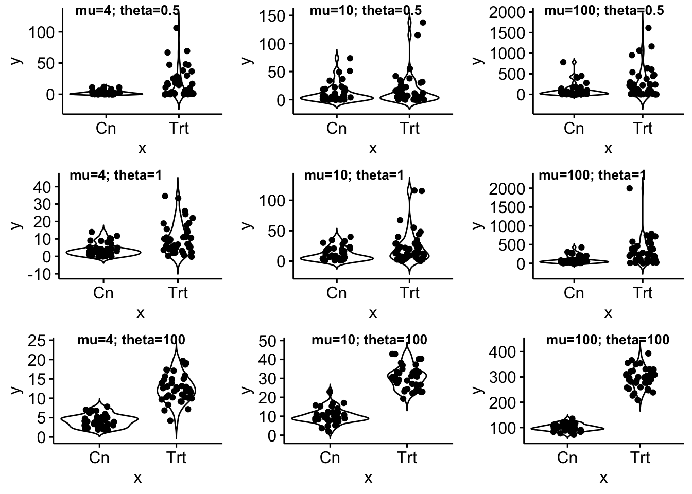

Type I error

res <- melt(res_table, 
            id.vars=c("beta_0", "beta_1", "n", "theta"),
            measure.vars=c("t", "Welch", "log", "Wilcoxan", "nb"),
            variable.name="model",
            value.name="frequency")
# res[, beta_0:=factor(beta_0)]
# res[, beta_1:=factor(beta_1)]
# res[, theta:=factor(theta)]
# res[, n:=factor(n)]

gg <- ggplot(data=res[beta_1==0], aes(x=n, y=frequency, group=model, color=model)) +
  geom_line() +
  facet_grid(beta_0 ~ theta, labeller=label_both) +
  NULL
gg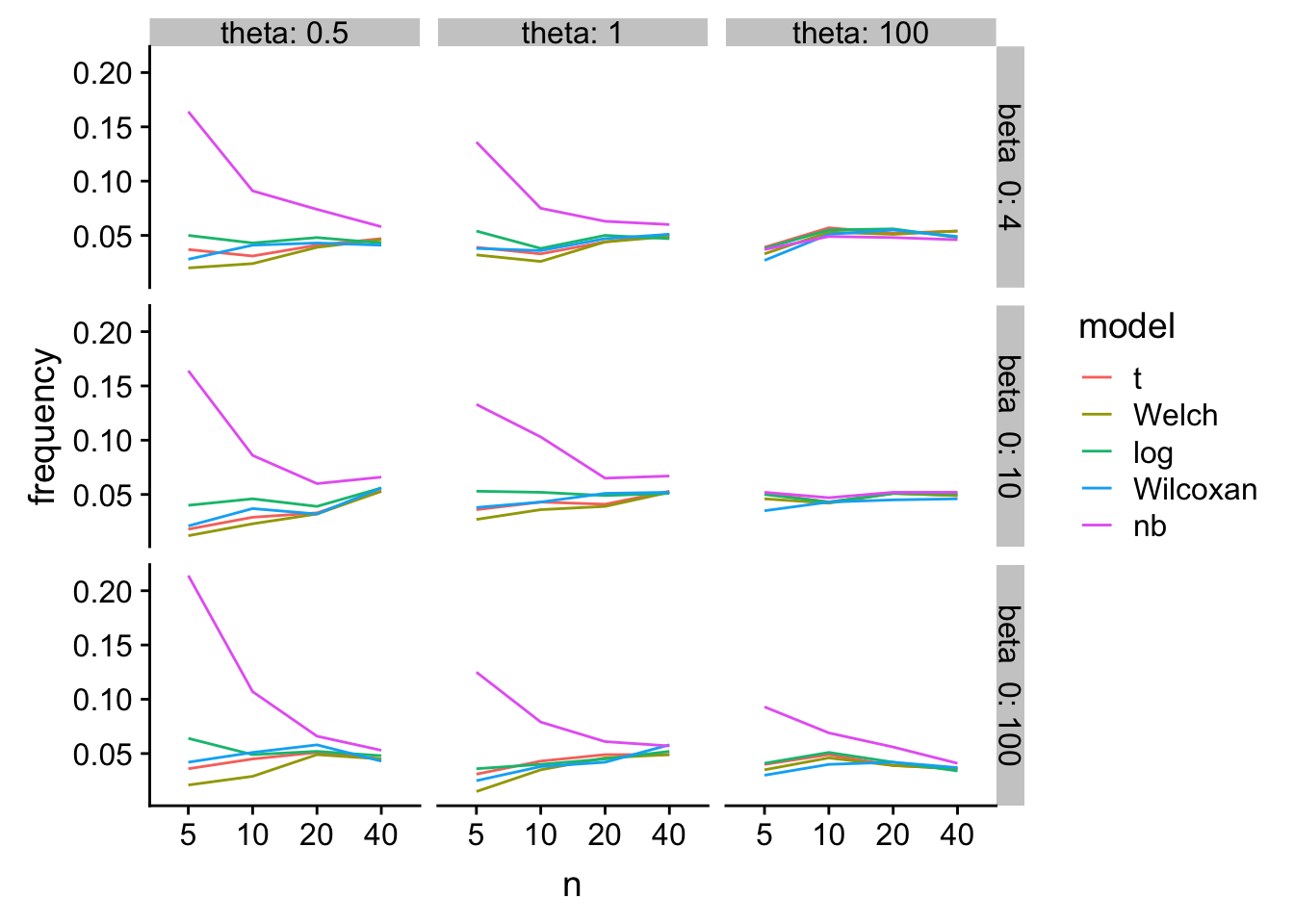

Ouch. glm-nb with hih error rates especially when n is small and the scale parameter is small

Power

b0_levels <- unique(res$beta_0)
# small count
gg1 <- ggplot(data=res[beta_0==b0_levels[1] & beta_1 > 0], aes(x=n, y=frequency, group=model, color=model)) +
  geom_line() +
  facet_grid(beta_1 ~ theta, labeller=label_both) +
  NULL

# large count
gg2 <- ggplot(data=res[beta_0==b0_levels[3] & beta_1 > 0], aes(x=n, y=frequency, group=model, color=model)) +
  geom_line() +
  facet_grid(beta_1 ~ theta, labeller=label_both) +
  NULL

gg1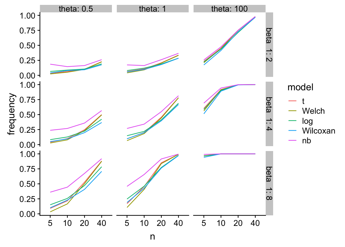

gg2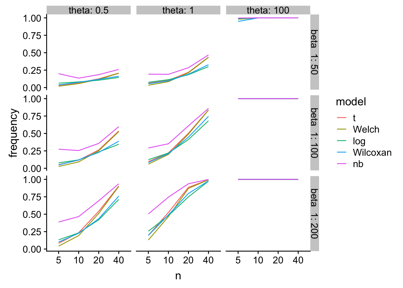

glm-nb has higher power, especially at small n, but at a type I cost.

GLM vs. t-tests vs. non-parametric tests if all we care about is NHST

load libraries

The simulation

Type I error

Power

R doodles. Some ecology. Some physiology. Much fake data.

GLM vs. t-tests vs. non-parametric tests if all we care about is NHST

load libraries

The simulation

Type I error

Power

R doodles. Some ecology. Some physiology. Much fake data.

How to make plots with factor levels below the x-axis (bench-biology style)

What is an interaction?

How to estimate synergism or antagonism

Type 3 ANOVA in R -- an easy way to publish wrong tables

Linear models with a covariate ("ANCOVA")

Normal Q-Q plots - what is the robust line and should we prefer it?

ANCOVA when the covariate is a mediator affected by treatment

Bootstrap confidence intervals when sample size is really small

What is the consequence of normalizing by each case in the control?

Melting a list of columns