
Should we be skeptical of a "large" effect size if p > 0.05?
Motivator: A twitter comment “Isn’t the implication that the large effect size is a direct byproduct of the lack of power? i.e. that if the the study had more power, the effect size would have been found to be smaller.”1 2
A thought: our belief in the magnitude of an observed effect should be based on our priors, which, hopefully, are formed from good mechanistic models and not sample size“.3
- If we observe a large effect but the sample size is small, then should we believe that the effect is strongly inflated?
- If we had measured a larger sample, would the effect be smaller?
But…maybe sample size should influence our prior, because the expected estimated effect magnitude is bigger than than the true effect if the true effect is near zero explored a bit here. This is because, if an effect is near zero, estimates will vary on both sides of zero, and the absolute value of most of these estimates will be bigger than the absolute value of the true effect. But what effect size should we worry about this?
Set up
library(ggplot2)
library(ggpubr)
## Loading required package: magrittrlibrary(data.table)The simulation
Simulate an experiment with two treatment levels (“control” and “treated”), with standardized (\(\frac{\delta}{\sigma}\)) effect sizes of 0.05, .1, .2, .3, .5, .8, 1, 2 and sample sizes of 100, 20, and 10. Cohen considered .8 a “large” standardized effect but I’ll leave what is large up to you. Regardless, its worth comparing the results here to observed effects.
n <- 100 # per treatment level. power will be a function of effect size
b_array <- c(0.05, 0.1, 0.2, 0.3, 0.5, 0.8, 1, 2)
niter <- 10^4
res_table <- data.table(NULL)
power_table <- data.table(NULL)
for(b1 in b_array){
  y1 <- matrix(rnorm(n*niter), nrow=n)
  y2 <- matrix(rnorm(n*niter), nrow=n) + b1
  d100 <- apply(y2, 2, mean) - apply(y1,2,mean)
  d20 <- apply(y2[1:20,], 2, mean) - apply(y1[1:20,],2,mean)
  d10 <- apply(y2[1:10,], 2, mean) - apply(y1[1:10,],2,mean)
  res_table <- rbind(res_table, data.table(b=b1, d100=d100, d20=d20, d10=d10))
  power_table <- rbind(power_table, data.table(
    b=b1,
    "power (n=100)"=power.t.test(n=100, delta=b1, sd=1)$power,
    "power (n=20)"=power.t.test(n=20, delta=b1, sd=1)$power,
    "power (n=10)"=power.t.test(n=10, delta=b1, sd=1)$power
  ))
}
Power for each simulation combination
knitr::kable(power_table, digits=2)| b | power (n=100) | power (n=20) | power (n=10) |
|---|---|---|---|
| 0.05 | 0.05 | 0.04 | 0.03 |
| 0.10 | 0.10 | 0.05 | 0.04 |
| 0.20 | 0.29 | 0.09 | 0.06 |
| 0.30 | 0.56 | 0.15 | 0.09 |
| 0.50 | 0.94 | 0.34 | 0.18 |
| 0.80 | 1.00 | 0.69 | 0.39 |
| 1.00 | 1.00 | 0.87 | 0.56 |
| 2.00 | 1.00 | 1.00 | 0.99 |
Absolute median effects
knitr::kable(res_table[, .("median(|b|) (n=100)"=median(abs(d100)),
              "median(|b|) (n=20)"=median(abs(d20)),
              "median(|b|) (n=10)"=median(abs(d10))
), by=b], digits=c(2, 3, 3, 3))| b | median(|b|) (n=100) | median(|b|) (n=20) | median(|b|) (n=10) |
|---|---|---|---|
| 0.05 | 0.100 | 0.212 | 0.302 |
| 0.10 | 0.121 | 0.224 | 0.308 |
| 0.20 | 0.197 | 0.260 | 0.332 |
| 0.30 | 0.299 | 0.318 | 0.370 |
| 0.50 | 0.501 | 0.502 | 0.515 |
| 0.80 | 0.799 | 0.796 | 0.792 |
| 1.00 | 1.000 | 0.993 | 0.995 |
| 2.00 | 2.001 | 2.004 | 2.002 |
Inflation factors
knitr::kable(res_table[, .(
              "IF (n=100)" = median(abs(d100))/b,
              "IF (n=20)" = median(abs(d20))/b,
              "IF (n=10)" = median(abs(d10))/b
), by=b], digits=c(2, 1, 1, 1))| b | IF (n=100) | IF (n=20) | IF (n=10) |
|---|---|---|---|
| 0.05 | 2.0 | 4.2 | 6.0 |
| 0.10 | 1.2 | 2.2 | 3.1 |
| 0.20 | 1.0 | 1.3 | 1.7 |
| 0.30 | 1.0 | 1.1 | 1.2 |
| 0.50 | 1.0 | 1.0 | 1.0 |
| 0.80 | 1.0 | 1.0 | 1.0 |
| 1.00 | 1.0 | 1.0 | 1.0 |
| 2.00 | 1.0 | 1.0 | 1.0 |
Directly answering question #2
Notice that if power is obove about .2, the absolute median effect is not inflated. That is, a study would have to be wicked underpowered for there to be an expected inflated effect size. This is an indirect answer to question no. 2. A more direct answer is explored by computing the log10 ratio of absolute effects between sample size levels for each run of the simulation.
res_table[, d100.d20:=log10(abs(d20)/abs(d100))]
res_table[, d100.d10:=log10(abs(d10)/abs(d100))]
res_table[, d20.d10:=log10(abs(d10)/abs(d20))]
res_melt <- melt(res_table[, .SD, .SDcols=c("b", "d100.d20", "d100.d10", "d20.d10")], id.vars="b", variable.name="comparison", value.name="contrast")
res_melt[, b:=factor(b)]
pd <- position_dodge(0.8)
ggplot(data=res_melt, aes(x=b, y=contrast, fill=comparison)) +
  geom_boxplot(position=pd, outlier.shape=NA) +
  coord_cartesian(ylim=c(-1.25, 2))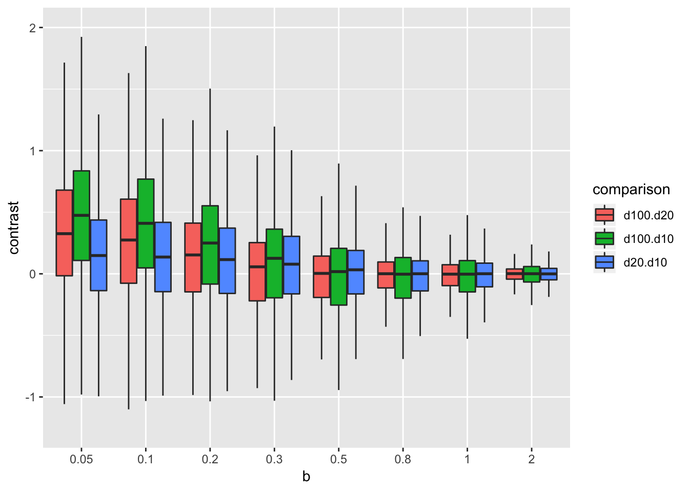
If the true effect is really small (0.05) then a smaller sample will often estimate a larger effect (just less than 75% of the time when decreasing \(n\) from 100 to 20). When the true effect is about 0.5 or higher, decreasing sample size is no more likely to estimate a bigger effect than increasing sample size.
The original question, and the motivating tweet, raise the question of what a “large” effect is. There is large in the absolute since, which would require subject level expertise to identify, and large relative to noise.↩
Note that the original post was not about the statistical significance filter but about the ethics of a RCT in which the observed effect was “large” but there was not enough power to get a statistically significant p-value.↩
at least if we are using an experiment to estimate an effect. If we are trying to estimate multiple effects, the bigger observed effects have tend to be inflated and the smaller observed effects tend to be dd↩
