
Using Wright's rules and a DAG to compute the bias of an effect when we measure proxies for X and Y
This is a skeletal post to work up an answer to a twitter question using Wright’s rules of path models. Using this figure
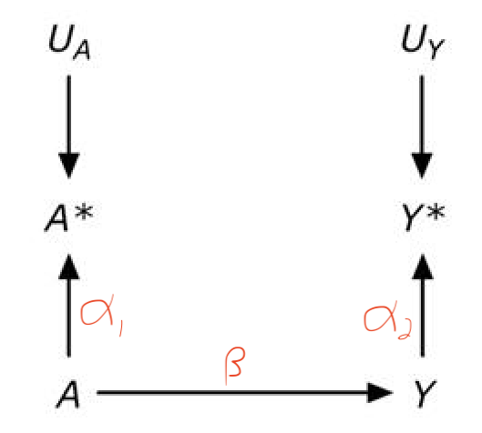
from Panel A of a figure from Hernan and Cole. The scribbled red path coefficients are added
the question is I want to know about A->Y but I measure A* and Y*. So in figure A, is the bias the backdoor path from A* to Y* through A and Y?
Short answer: the bias is the path as stated divided by the path from A to Y.
Medium answer: We want to estimate \(\beta\), the true effect of \(A\) on \(Y\). We have measured the proxies, \(A^\star\) and \(Y^\star\). The true effect of \(A\) on \(A^\star\) is \(\alpha_1\) and the true effect of \(Y\) on \(Y^\star\) is \(\alpha_2\).
So what we want is \(\beta\) but what we estimate is \(\alpha_1 \beta \alpha_2\) (the path from \(A^\star\) to \(Y^\star\)) so the bias is \(\alpha_1 \alpha_2\).
But, this is really only true for standardized effects. If the variables are not variance-standardized (and why should they be?), the bias is a bit more complicated.
TL;DR answer: In terms of \(\beta\) the estimated effect is
\[\begin{equation} \alpha_1 \alpha_2 \frac{\sigma_A^2}{\sigma_{A^\star}^2} \beta \end{equation}\]so the bias is
\[\begin{equation} k = \alpha_1 \alpha_2 \frac{\sigma_A^2}{\sigma_{A^\star}^2} \end{equation}\]The derivation is scratched out here:
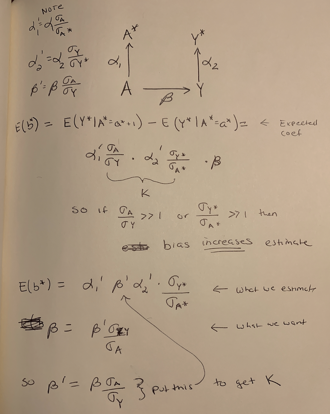
Old fashion doodle deriving the bias of the estimate of \(\beta\) when proxies of A and Y are measured. The bias is k.
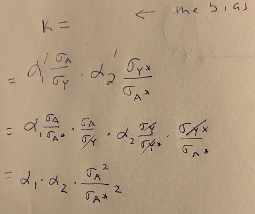
Part 2 of the derivation. Substituting the non-standardized coefficients in for the standardized coefficients.
If the data are standardized (all variables have unit variance)
This is easy and just uses Wright’s rules of adding up effects along a path
n <- 10^6
beta <- 0.6 # true effect
alpha_1 <- 0.9 # standardized effect of A on A* -- this is the correlation of A with proxy
alpha_2 <- 0.8 # standardized effect of Y o Y* -- this is the correlation of Y with proxy
A <- rnorm(n)
Y <- beta*A + sqrt(1 - beta^2)*rnorm(n)
astar <- alpha_1*A + sqrt(1 - alpha_1^2)*rnorm(n) # proxy for A
ystar <- alpha_2*Y + sqrt(1 - alpha_2^2)*rnorm(n) # proxy for Y
\(\beta\) is the true effect and the expected estimated effect is \(\alpha_1 \beta \alpha_2\) (using Wright rules) so \(\alpha_1 \alpha_2\) is the bias. Note this isn’t added to the true effect as in omitted variable bias (confounding). We can check this with the fake data.
alpha_1*beta*alpha_2 # expected measured effect## [1] 0.432coef(lm(ystar ~ astar)) # measured effect## (Intercept) astar
## 0.0007277386 0.4313778378check some other measures
var(A) # should be 1## [1] 1.002161var(Y) # should be 1## [1] 1.001362var(astar) # should be 1## [1] 1.00204var(ystar) # should be 1## [1] 0.998893cor(ystar, astar) # should be equal to expected measured effect## [1] 0.4320569if the data are not standardized
n <- 10^5
rho_alpha_1 <- 0.9 # correlation of A and A*
rho_alpha_2 <- 0.8 # correlation of Y and Y*
rho_b <- 0.6 # standardized true effect of A on Y
sigma_A <- 2 # total variation in A
sigma_Y <- 10 # total variation in Y
sigma_astar <- 2.2 # total variation in A*
sigma_ystar <- 20 # total variation in Y*
alpha_1 <- rho_alpha_1*sigma_astar/sigma_A # effect of A on astar
alpha_2 <- rho_alpha_2*sigma_ystar/sigma_Y # effect of Y on ystar
beta <- rho_b*sigma_Y/sigma_A # effect of A on Y (the thing we want)
A <- rnorm(n, sd=sigma_A)
R2_Y <- (beta*sigma_A)^2/sigma_Y^2 # R^2 for E(Y|A)
Y <- beta*A + sqrt(1-R2_Y)*rnorm(n, sd=sigma_Y)
R2_astar <- (alpha_1*sigma_A)^2/sigma_astar^2 # R^2 for E(astar|A)
astar <- alpha_1*A + sqrt(1-R2_astar)*rnorm(n, sd=sigma_astar)
R2_ystar <- (alpha_2*sigma_Y)^2/sigma_ystar^2 # R^2 for E(ystar|Y)
ystar <- alpha_2*Y + sqrt(1-R2_ystar)*rnorm(n, sd=sigma_ystar)
Now let’s check our math in the figure above. Here is the estimated effect
coef(lm(ystar ~ astar))## (Intercept) astar
## 0.004357835 3.950256435And the expected estimated effect using just the standardized coefficients
rho_alpha_1*rho_alpha_2*rho_b*sigma_ystar/sigma_astar## [1] 3.927273And the expected estimated effect using the equation \(k \beta\), where k is the bias (this is in the top image of the derivation)
k <- rho_alpha_1*sigma_A/sigma_Y*rho_alpha_2*sigma_ystar/sigma_astar
k*beta
## [1] 3.927273And finally, the expected estimated effect using the bias as a function of the unstandardized variables (this is in the bottom – part 2– image of the derivation)
k <- alpha_1*alpha_2*sigma_A^2/sigma_astar^2
k*beta
## [1] 3.927273And the true effect?
beta## [1] 3Some other checks
coef(lm(ystar ~ Y))## (Intercept) Y
## -0.03612649 1.60271514alpha_2## [1] 1.6coef(lm(ystar ~ A))## (Intercept) A
## -0.00254846 4.80956599alpha_2*beta## [1] 4.8coef(lm(astar ~ A))## (Intercept) A
## -0.002796505 0.991465329alpha_1## [1] 0.99sd(A)## [1] 2.014547sd(Y)## [1] 10.04232sd(astar)## [1] 2.215202sd(ystar)## [1] 20.09823cor(A, astar)## [1] 0.9016573cor(Y, ystar)## [1] 0.8008157```
